
Prompting is used in vision models for segmentation, object identification, and image synthesis. The model prompts could be text, pixel coordinates, bounding boxes, or segmentation.
In this course, we will instruct the S.A.M. model to recognize an object's outline by providing it with coordinates, points, or bounding boxes. You can also use a negative prompt to indicate something you don't want.
The number of inference step hyperparameters determines how gradually the model transforms a noisy distribution into a clean one. More stages generally result in more detailed and accurate creation because the model has more possibilities to modify the data. However, additional stages require greater computation time. The strength hyperparameter and the context of stable diffusion determine how noisy the initial distribution is during the inpainting process, where the added noise is used to erase portions of the initial image. In essence, strength determines how much of the initial image is retained in the diffusion process.
To modify the stable diffusion model to correlate a text label with a specific item, such as your good friend, we will employ Google Research's Dreambooth finetuning approach.
Image Segmentation
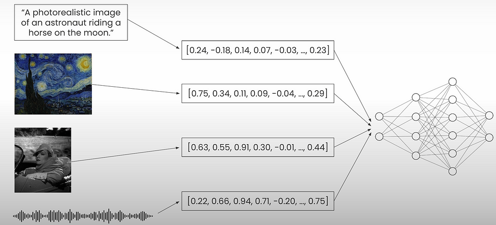
A prompt is just an input that directs output distribution; thus, it can be text, image, video, or audio.
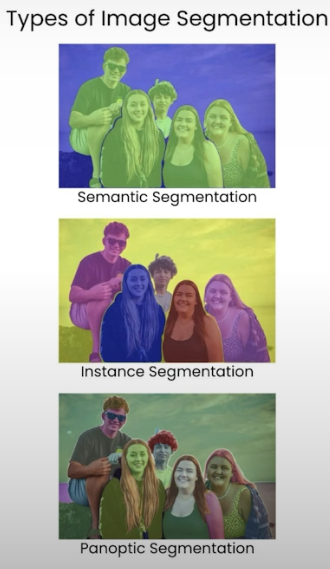
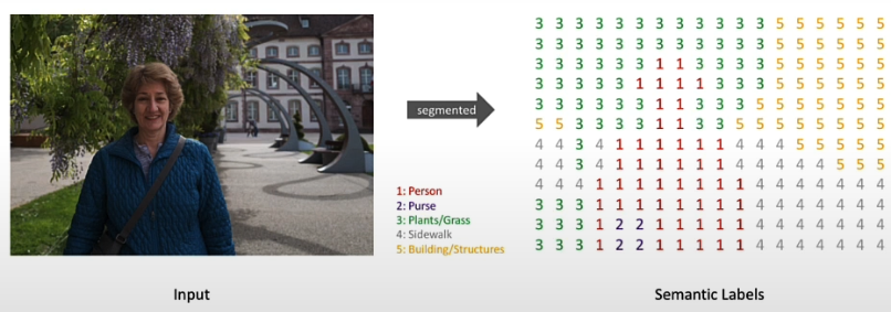
More precisely, image segmentation is the process of giving a label to each pixel in a picture so that pixels with the same label have specific properties. In this episode, we'll look at the Segment Anything Model, prompting using pixel coordinates, prompting with multiple sets of coordinates, prompting with bounding boxes, and using both a positive and a negative prompt.
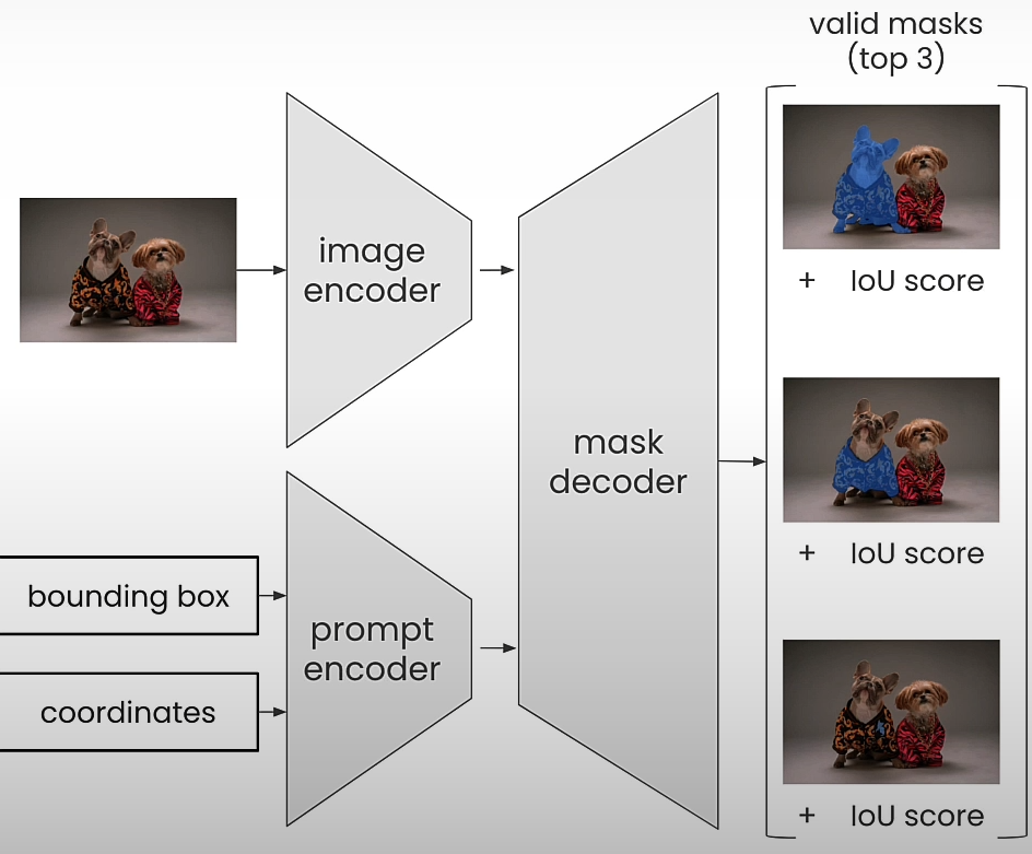
The original Segment Anything Model is a computer vision milestone that has served as the foundation for several high-level downstream tasks such as picture segmentation, captioning, and editing. However, its high processing costs limit its use in industry contexts such as edge devices. The majority of SAM's computing costs are due to its transformer architecture. As shown in the graphic above, SAM accepts image bounding box coordinates, single-pixel coordinates, and an input image. Each of these inputs is encoded by either an image encoder or a prompt encoder. They are then passed into the masked decoder, where SAM returns the top three valid masks for the given point or bounding box.
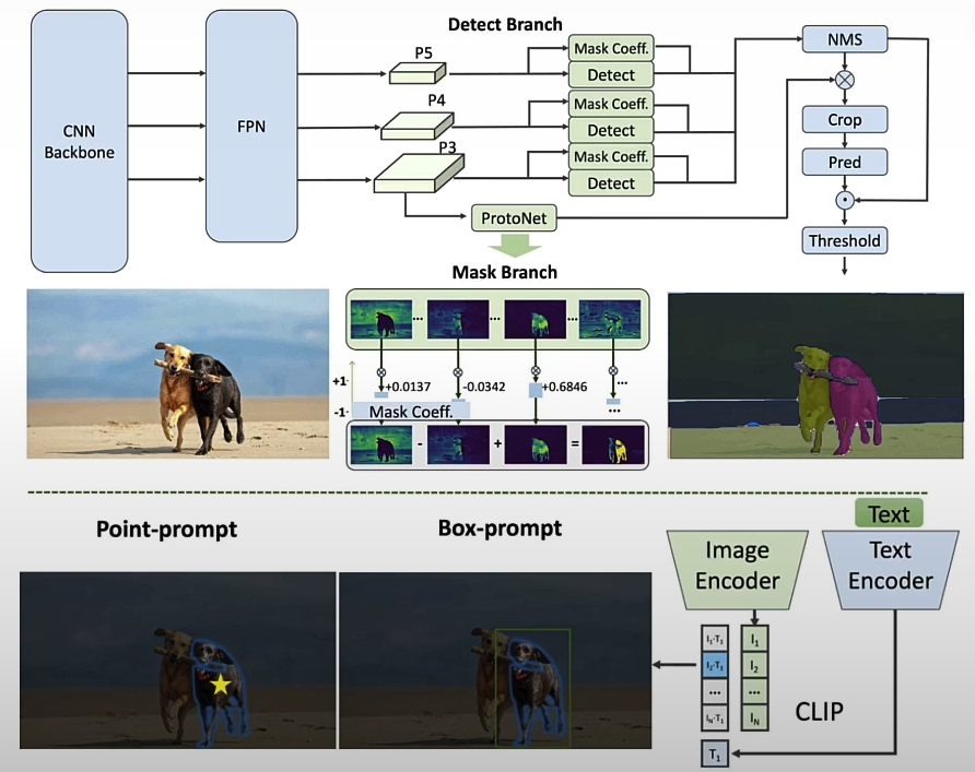
The FASTSAM is a CNN-based model trained with only 2% of the original data set published by the SAM authors, and it achieves comparable performance on 32x32 images while running at 50 times the speed. Prompting rapid SAM differs somewhat from prompting the original SAM. It automatically discovers all masks in an image that above a specified confidence level and then filters all created masks depending on the user-provided prompts.
#Load the sample image
from PIL import Image
raw_image = Image.open("dogs.jpg")
raw_image

# Resize the image
from utils import resize_image
resized_image = resize_image(raw_image, input_size=1024)
resized_image

# Import and prepare the model
import torch
device = torch.device("cuda" if torch.cuda.is_available() else "cpu")
device

from ultralytics import YOLO
model = YOLO('./models/comet-c1/FastSAM.pt')

# Using the model
from utils import show_points_on_image
# Define the coordinates for the point in the image
# [x_axis, y_axis]
input_points = [ [350, 450 ] ]
input_labels = [1] # positive point
# Function written in the utils file
show_points_on_image(resized_image, input_points)
# Run the model
results = model(resized_image, device=device, retina_masks=True)

# Filter the mask based on the point defined before
from utils import format_results, point_prompt
results = format_results(results[0], 0)
# Generate the masks
masks, _ = point_prompt(results, input_points, input_labels)
from utils import show_masks_on_image
# Visualize the generated masks
show_masks_on_image(resized_image, [masks])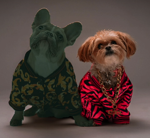
# Define semantic masks two points to be masked
# Specify two points in the same image
# [x_axis, y_axis]
input_points = [ [350, 450], [620, 450] ]
# Specify both points as "positive prompt"
input_labels = [1 , 1] # both positive points
# Visualize the points defined before
show_points_on_image(resized_image, input_points)
# Run the model
results = model(resized_image, device=device, retina_masks=True)
results = format_results(results[0], 0)
# Generate the masks
masks, _ = point_prompt(results, input_points, input_labels)
# Visualize the generated masks
show_masks_on_image(resized_image, [masks])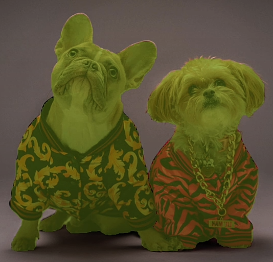
# Identify subsections of the image by adding a negative prompt
# Define the coordinates for the regions to be masked
# [x_axis, y_axis]
input_points = [ [350, 450], [400, 300]  ]
input_labels = [1, 0] # positive prompt, negative prompt
# Visualize the points defined above
show_points_on_image(resized_image, input_points, input_labels)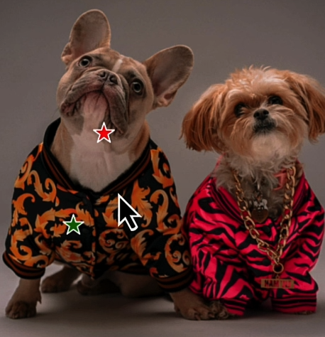
# Note: From the image above, the red star indicates the negative prompt and the green star the positive prompt.
# Run the model
results = model(resized_image, device=device, retina_masks=True)
results = format_results(results[0], 0)
# Generate the masks
masks, _ = point_prompt(results, input_points, input_labels)
# Visualize the generated masks
show_masks_on_image(resized_image, [masks])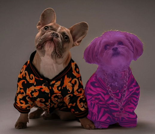
# Prompting with bounding boxes
from utils import box_prompt
# Set the bounding box coordinates
# [xmin, ymin, xmax, ymax]
input_boxes = [530, 180, 780, 600]
from utils import show_boxes_on_image
# Visualize the bounding box defined with the coordinates above
show_boxes_on_image(resized_image, [input_boxes])

# Now try to isolate the mask from the total output of the model
from utils import box_prompt
results = model(resized_image, device=device, retina_masks=True)
# Generate the masks
masks = results[0].masks.data
masks
# Convert to True/False boolean mask
masks = masks > 0
masks
masks, _ = box_prompt(masks, input_boxes)
# Visualize the masks
show_masks_on_image(resized_image, [masks])
# Print the segmentation mask, but in its raw format
masks
# To visualize, import matplotlib
from matplotlib import pyplot as plt
# Plot the binary mask as an image
plt.imshow(masks, cmap='gray')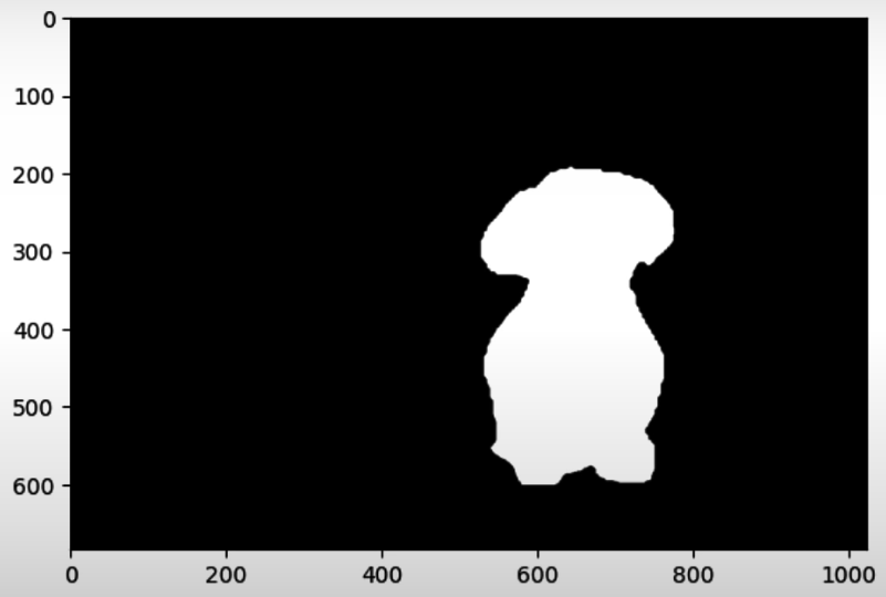
Additional Resources
- For more on using Comet for experiment tracking, check out this Quickstart Guide and the Comet Docs.
- This course was based on a set of two blog articles from Comet. Explore them here for more on how to use newer versions of Stable Diffusion in this pipeline, additional tricks to improve your inpainting results, and a breakdown of the pipeline architecture:
- SAM + Stable Diffusion for Text-to-Image Inpainting
- Image Inpainting for SDXL 1.0 Base Model + Refiner
Object Detection
Let's zero-shot. The model Owl-ViT, where ViT stands for vision transformer, is a zero-shot object detection model that does not require picture training. We will utilize the output of this model to feed into the SAM you used in the last lesson. We will build an image editing pipeline by connecting these two vision models such that a user can provide a prompt and the pipeline returns a segmentation mask.
The OWL-ViT model was trained in two phases: pre-training and fine-tuning. During the corresponding phase, the model learns to link an image with a piece of text using a contrastive loss technique, allowing the OWL-Vit model to build a deep knowledge of both the image and the text. To get good performance, this model has to be fine-tuned. At this level, the model is specially trained for object detection. While in the initial phase, the model was only learning how to correlate a piece of text with an image; in the fine-tuning stage, the model learns to identify objects and associate them with a specific word or string.
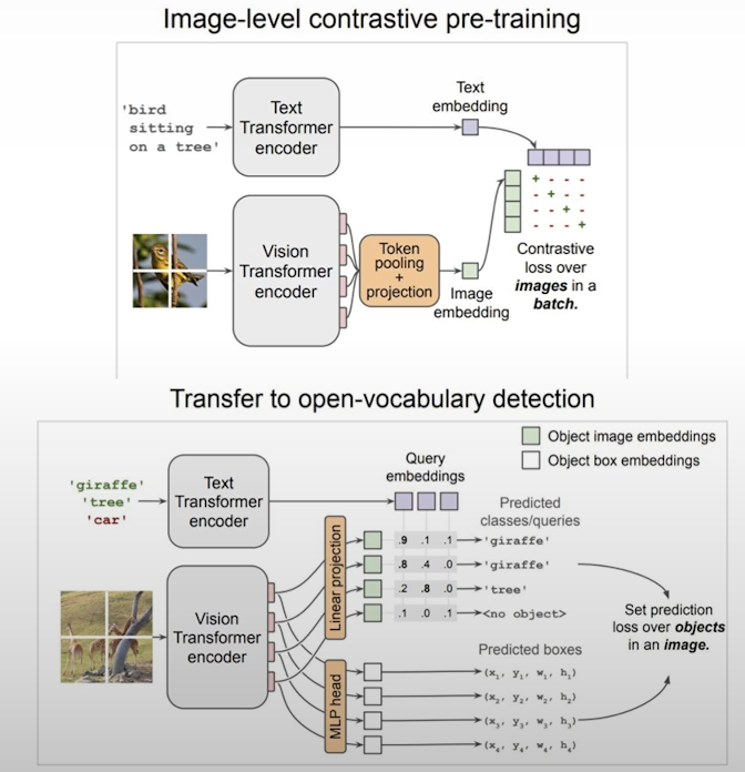
Before we apply the two models in this pipeline, let's set up a comet experiment to compare the generated masks at the end of the pipeline.
import comet_ml
comet_ml.login(anonymous=True, project_name="3: OWL-ViT + SAM") # anonymous require no account
exp = comet_ml.Experiment()

# To display the image
from PIL import Image
logged_artifact = exp.get_artifact("L3-data", "anmorgan24")

local_artifact = logged_artifact.download("./")
# Display the images
raw_image = Image.open("L3_data/dogs.jpg")
raw_image

# Getting bounding boxes with OWL-ViT object detection model
from transformers import pipeline
OWL_checkpoint = "./models/google/owlvit-base-patch32"

# Building the pipeline for the detector model
# Load the model
detector = pipeline(
    model= OWL_checkpoint,
    task="zero-shot-object-detection"
)
# What you want to identify in the image
text_prompt = "dog"
output = detector(
    raw_image,
    candidate_labels = [text_prompt]
)
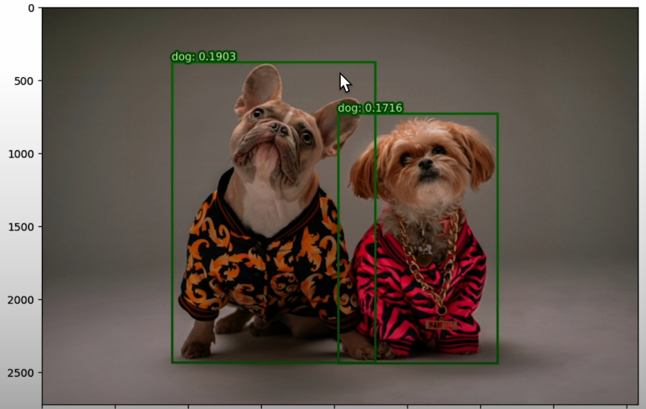
# Print the output to identify the bounding boxes detected
output

# Using utils function to prompt boxes in top of the image
from utils import preprocess_outputs
input_scores, input_labels, input_boxes = preprocess_outputs(output)
from utils import show_boxes_and_labels_on_image
# Show the image with the bounding boxes
show_boxes_and_labels_on_image(
    raw_image,
    input_boxes[0],
    input_labels,
    input_scores
)
We will use the MobileSAM model, which has been tuned to work on smartphones that may not have GPUs. To improve performance, the MobileSAM model employs a technique called as model distillation.
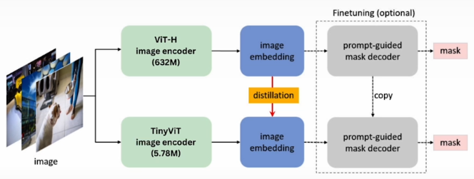
Model distillation is the process of moving information from a larger model to a smaller one. Model distillation differs from previous model compression approaches in that it does not modify the model format but instead creates a totally new and smaller model.
# Getting segmentation masks using Mobile SAM
# Load the SAM model from the imported ultralytics library
from ultralytics import SAM
SAM_version = "mobile_sam.pt"
model = SAM(SAM_version)

# Generating an array using numpy
import numpy as np
# Create a list of positive labels of same length as the number of predictions generated above
labels = np.repeat(1, len(output))
# Print the labels
print(labels) # array([1,1])
result = model.predict(
    raw_image,
    bboxes=input_boxes[0],
    labels=labels
)
print(result)
"""
0: 1024x1024 892.4ms
Speed: 19.6ms preprocess, 892.4ms inference, 24.9ms postprocess per image at
shape (1, 3, 1024, 1024)
"""
masks = result[0].masks.data
masks
from utils import show_masks_on_image
# Visualize the masks
show_masks_on_image(
    raw_image,
    masks
)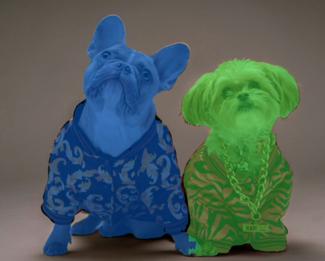
You successfully used the OWL model to move from a text prompt to a bending box and the SAM model to generate masks. Putting these together, we now have a pipeline that goes directly from text to masked image.
Let us try another use case in which we blur the faces of the persons.
from PIL import Image
image_path = "L3_data/people.jpg"
raw_image = Image.open(image_path)
print(raw_image)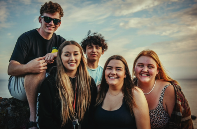
print(raw_image.size) # (9000, 6000)

# Calculate width percent to maintain aspect ratio in resize transformation
mywidth = 600
wpercent = mywidth / float(raw_image.size[0])
print(wpercent) # 0.066666666667

# Calculate height percent to maintain aspect ratio in resize transformation
hsize = int( float(raw_image.size[1]) * wpercent )
print(hsize) # 400

# Resize the image
raw_image = raw_image.resize([mywidth, hsize])

print(raw_image.size) # (600, 400)

# Save the resized image
image_path_resized = "people_resized.jpg"
raw_image.save(image_path_resized)

# Detecting faces
candidate_labels = ["human face"]
# Define a new Comet experiment for this new pipeline
exp = comet_ml.Experiment()
# Log raw image to the experiment
_ = exp.log_image(
    raw_image,
    name = "Raw image"
)

# Creating bounding boxes with OWL-ViT
# Apply detector model to the raw image
output = detector(
    raw_image,
    candidate_labels=candidate_labels
)
input_scores, input_labels, input_boxes = preprocess_outputs(output)
# Print values of the bounding box coordinates identified
input_boxes

# Log the images and bounding boxes
metadata = {
    "OWL prompt": candidate_labels,
    "SAM version": SAM_version,
    "OWL Version": OWL_checkpoint
}
from utils import make_bbox_annots
annotations = make_bbox_annots(
    input_scores,
    input_labels,
    input_boxes,
    metadata
)
_ = exp.log_image(
    raw_image,
    annotations= annotations,
    metadata=metadata,
    name= "OWL output"
)

# Segmentation masks using SAM
result = model.predict(
    image_path_resized,
    bboxes=input_boxes[0],
    labels=np.repeat(1, len(input_boxes[0]))
)

# First we blur the entire image
from PIL.ImageFilter import GaussianBlur
blurred_img = raw_image.filter(GaussianBlur(radius=5))
print(blurred_img)
masks = result[0].masks.data.cpu().numpy()
# Create an array of zeroes of the same shape as our image mask
total_mask = np.zeros(masks[0].shape)
# Add each output mask to the total_mask
for mask in masks:
    total_mask = np.add(total_mask,mask)
# Where there is any value other than zero (where any masks exist), show the blurred image
# Else, show the original (unblurred) image
output = np.where(
    np.expand_dims(total_mask != 0, axis=2),
    blurred_img,
    raw_image
)
import matplotlib.pyplot as plt
# Print image with faces blurred
plt.imshow(output)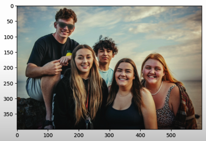
# Logging this image in the Comet platform
metadata = {
    "OWL prompt": candidate_labels,
    "SAM version": SAM_version,
    "OWL version": OWL_checkpoint
}
_ = exp.log_image(
    output,
    name="Blurred masks",
    metadata = metadata,
    annotations=None
)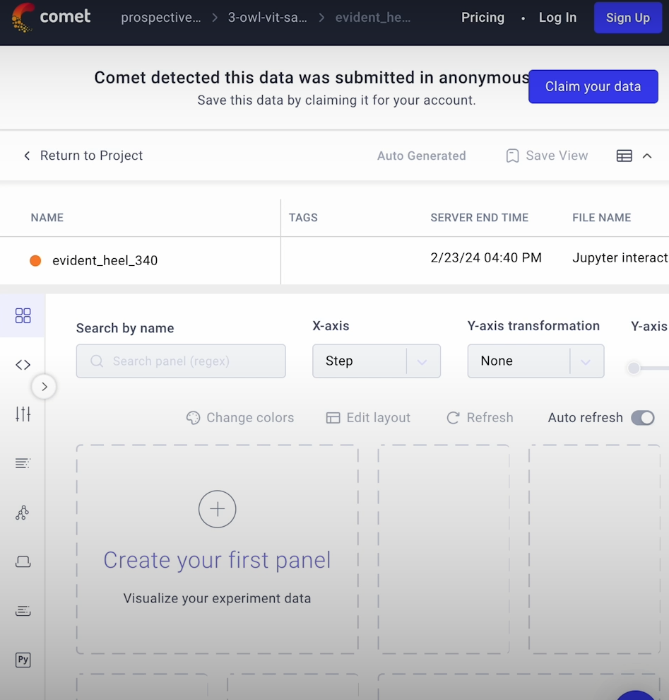
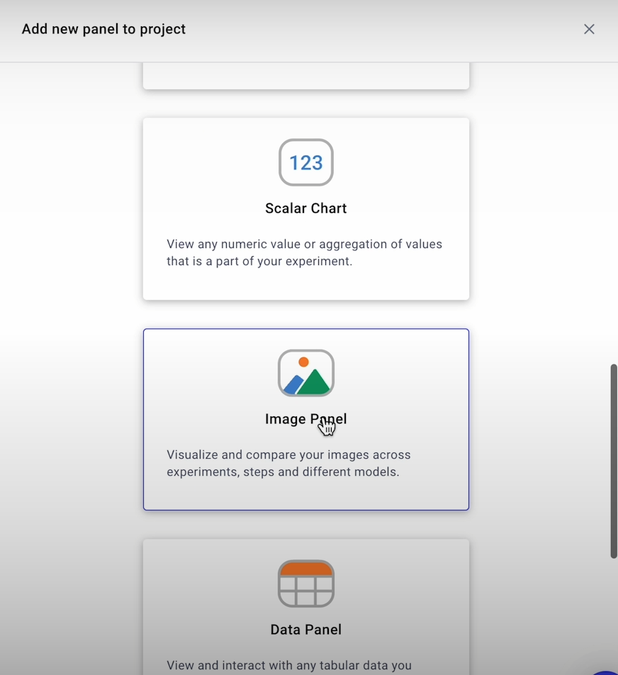
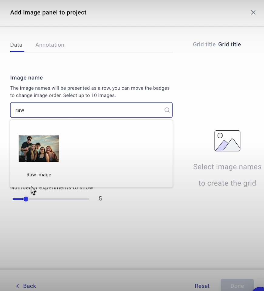
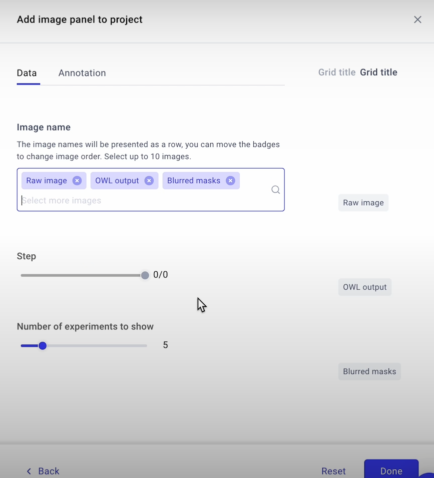
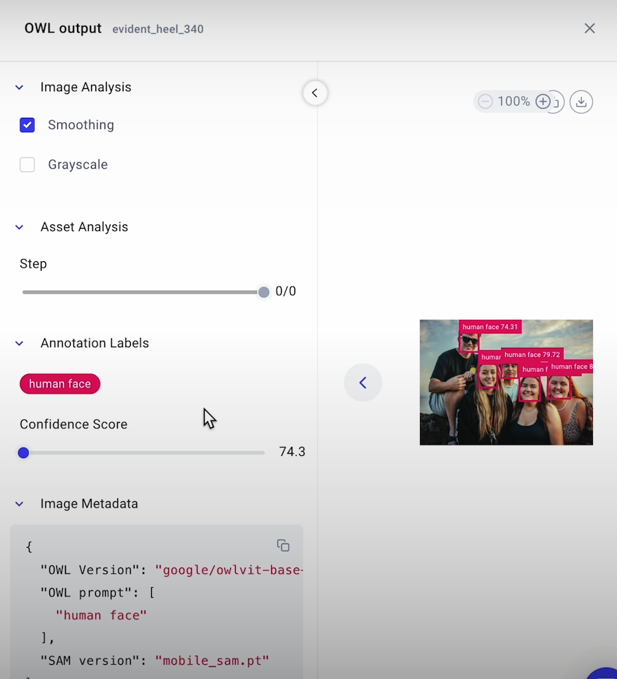
Let's look at the middle steps and debug our pipeline using the Comet platform.
# Blur just faces of those not wearing sunglasses
# New label
candidate_labels = ["a person without sunglasses"]
# Reruning the pipeline
exp = comet_ml.Experiment()
_ = exp.log_image(raw_image, name="Raw image")
output = detector(raw_image, candidate_labels=candidate_labels)
input_scores, input_labels, input_boxes = preprocess_outputs(output)
# Print the bounding box coordinates
print(input_boxes) # [[[125,49,190,79]]]

# Exploring what is happening in the Comet plaform
from utils import make_bbox_annots
metadata = {
    "OWL prompt": candidate_labels,
    "SAM version": SAM_version,
    "OWL version": OWL_checkpoint,
}
annotations = make_bbox_annots(
    input_scores,
    input_labels,
    input_boxes,
    metadata
)
_ = exp.log_image(
    raw_image,
    annotations=annotations,
    metadata=metadata,
    name="OWL output no sunglasses"
)
result = model.predict(
    image_path_resized,
    bboxes=input_boxes[0],
    labels=np.repeat(1, len(input_boxes[0]))
)
from PIL.ImageFilter import GaussianBlur
blurred_img = raw_image.filter(GaussianBlur(radius=5))
masks = result[0].masks.data.cpu().numpy()

total_mask = np.zeros(masks[0].shape)
for mask in masks:
    total_mask = np.add(total_mask, mask)
# Print the result
output = np.where(
    np.expand_dims(total_mask != 0, axis=2),
    blurred_img,
    raw_image
)
plt.imshow(output)

# Analyzing results in the Comet plaform
metadata = {
    "OWL prompt": candidate_labels,
    "SAM version": SAM_version,
    "OWL version": OWL_checkpoint,
}
_ = exp.log_image(
    output,
    name="Blurred masks no sunglasses",
    metadata=metadata,
    annotations=None
)

# Trying yourself
cafe_img = Image.open("L3_data/cafe.jpg")
cafe_img
crosswalk_img = Image.open("L3_data/crosswalk.jpg")
crosswalk_img
metro_img = Image.open("L3_data/metro.jpg")
metro_img
friends_img = Image.open("L3_data/friends.jpg")
friends_img
Additional Resources
- For more on using Comet for experiment tracking, check out this Quickstart Guide and the Comet Docs.
- This course was based on a set of two blog articles from Comet. Explore them here for more on how to use newer versions of Stable Diffusion in this pipeline, additional tricks to improve your inpainting results, and a breakdown of the pipeline architecture:
- SAM + Stable Diffusion for Text-to-Image Inpainting
- Image Inpainting for SDXL 1.0 Base Model + Refiner
Image Generation
Stable diffusion models can be prompted using text, graphics, or masks. You can also adjust some hyperparameters, such as guidance, scale, strength, and the number of inference steps, to better manage the diffusion process. Let's look at how vision models can be used to add information to images through diffusion models. Before we get started, let's look at how diffusion models function behind the scenes.
Diffusion models convert a picture of random noise into a target image. The model produces a picture with pure Gaussian noise. The model then gradually denoises the image one step at a time, until we have an image with no noise. You can think of it as if we are lying about the model by including an image of a dog within a noise where there is only noise. A U-Net is used to gradually denoise an image across multiple timesteps. A text encoder generates prompt embeddings that help the denoising process.

Models can accept more than just text; you can also input images, masks, and numerous hyperparameters to help control the diffusion process. You may even instruct your model to take an initial image and then use diffusion to alter only a piece of it using a method known as inpainting.
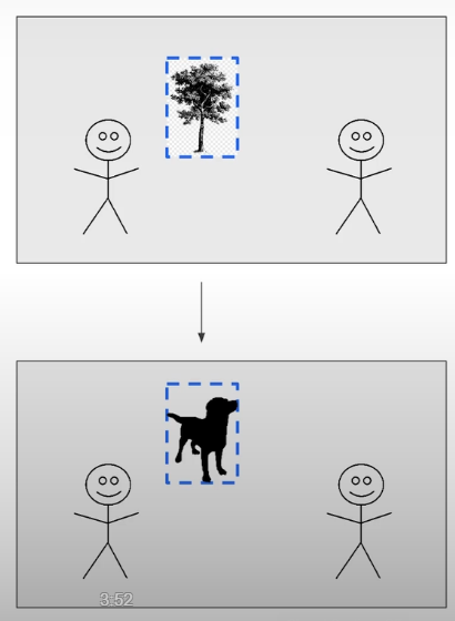
To get started, we will download our masks and photos from Comet as artifacts. Artifacts are just version-controlled assets. Artifacts include models, datasets, pictures, and a segmentation mask of a cat. Once we have downloaded the artifact, we can extract the photos and view them with matplotlib.
import comet_ml
comet_ml.login(anonymous=True, project_name="4: Diffusion Prompting")
# Create the Comet Experiment for logging
exp = comet_ml.Experiment()

logged_artifact = exp.get_artifact("L4-data", "anmorgan24")
local_artifact = logged_artifact.download("./")

# Loading images
from PIL import Image
image=Image.open("L4_data/boy-with-kitten.jpg").resize((256, 256))
image_mask=Image.open("L4_data/cat_binary_mask.png").resize((256, 256))

import matplotlib.pyplot as plt
# Print the image
plt.imshow(image)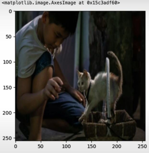
# Print the mask
plt.imshow(image_mask)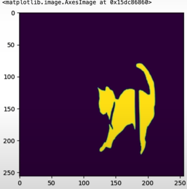
# Import and prepare the model
import torch
device = torch.device("cuda" if torch.cuda.is_available() else "cpu")

from diffusers import StableDiffusionInpaintPipeline
sd_pipe = StableDiffusionInpaintPipeline.from_pretrained(
    "./models/stabilityai/stable-diffusion-2-inpainting",
    torch_dtype=torch.float16 if torch.cuda.is_available() else torch.bfloat16,
    low_cpu_mem_usage=False if torch.cuda.is_available() else True,
).to(device)

# Set the value of seed manually for reproducibility of the results
seed = 66733
generator = torch.Generator(device).manual_seed(seed)

prompt = "a realistic green dragon"
More inference stages indicate a more gradual denoising process, resulting in higher-quality photos. Too many stages waste computing resources and can result in overprocessed photos.
Initiate the Stable Diffusion inpainting process.If you'd like to learn more about the float16 versus bfloat16 data types and when you'd utilize one over the other, then check out the following short course:
"Quantization Fundamentals" Lesson "Data Types and Sizes
Hardware requirements: A system with at least 8 GB of CPU should enough to generate the images taught in this lab, with results expected in about 3 minutes for three inference stages. However, for operations with ten steps, employing a CPU may increase execution time to around ten minutes. Tasks with 100 steps will greatly increase the execution time on a CPU. Alternatively, consider using a GPU to accelerate processing. All three stages can be accomplished in less than a second using a GPU, such as a local one or a platform like Colab.
# Define new Comet experiment
"""
The following image generation code will takes hours without a GPU.
Its results are saved with an experiment tracking tool (Comet), so that you can retrieve them in this classroom environment (and on any computer, regardless of GPU access).
"""

exp = comet_ml.Experiment()

output = sd_pipe(
  image=image,
  mask_image=image_mask,
  prompt=prompt,
  generator=generator,
  num_inference_steps=3,
)
generated_image = output.images[0]

exp.log_image(
    generated_image,
    name=f"{prompt}",
    metadata={
        "prompt": prompt,
        "seed": seed,
        "num_inference_steps": 3
    }
)

exp.end()

# Retrieve the experiment results
"""
Regardless of the environment that you are running in, you can retrieve the results of the experiment using the experiment tracking tool (Comet).
"""
import io

reference_experiment = comet_ml.APIExperiment(
    workspace="ckaiser",
    project_name="4-diffusion-prompting",
    previous_experiment="b1b9e80bb0054b52a8914beec97d36a6"
)

reference_image = reference_experiment.get_asset_by_name(f"{prompt}")

# Print the reference_image
plt.imshow(Image.open(io.BytesIO(reference_image)))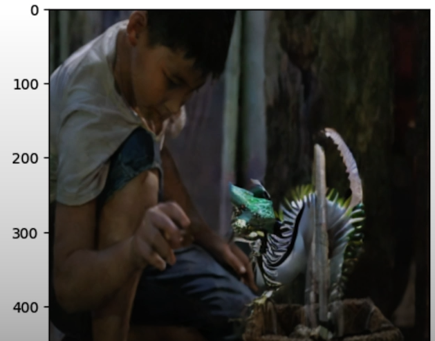
# Let's explore different hyperparameters. Set up a different 'number of inference steps'.
# Below code NEEDS GPU
exp = comet_ml.Experiment()

prompt = "a realistic green dragon"

exp.log_parameters({
    "seed": seed,
    "num_inference_steps": 100
})
output = sd_pipe(
  image=image,
  mask_image=image_mask,
  prompt=prompt,
  generator=generator,
  num_inference_steps=100,
)

generated_image = output.images[0]

exp.log_image(
    generated_image,
    name=f"{prompt}",
    metadata={
        "prompt": prompt,
        "seed": seed,
        "num_inference_steps": 100
    }
)

exp.end()

# Return the experiment results
reference_experiment = comet_ml.APIExperiment(
    workspace="ckaiser",
    project_name="4-diffusion-prompting",
    previous_experiment="948c8e6cfd23420c86a0de5f65719955"
)

reference_image = reference_experiment.get_asset_by_name(f"{prompt}")
plt.imshow(Image.open(io.BytesIO(reference_image)))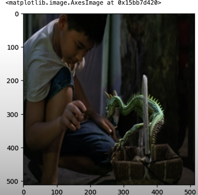
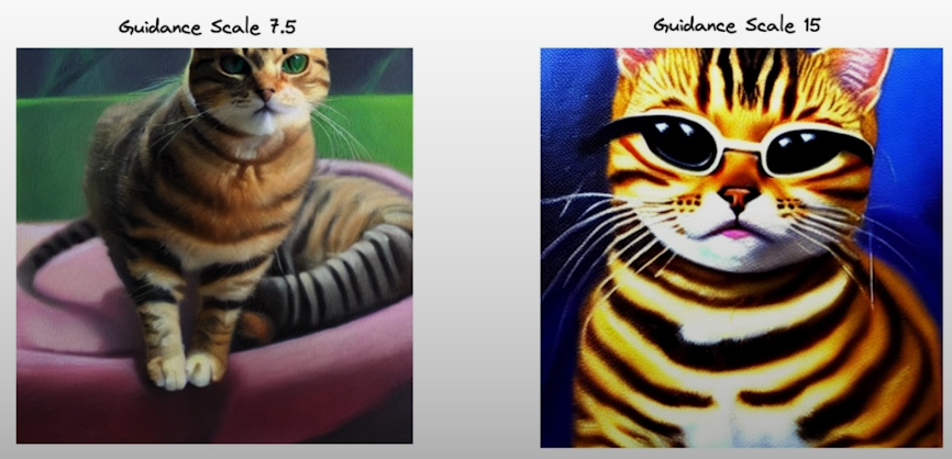
The Guidance Scale is a numerical value that indicates how closely the model should follow the prompts. A higher guidance scale indicates greater prompt fidelity, but potentially lesser image quality. The default guiding scale value varies depending on the diffusion model.
# Set up the different 'Guidance Scale' values. (BELOW CODE NEEDS GPU)
import numpy as np
guidance_scale_values = [x for x in np.arange(0, 21, 10)]
exp = comet_ml.Experiment()

prompt = "a realistic green dragon"

num_inference_steps = 100 #if torch.cuda.is_available() else 10

exp.log_parameters({
    "seed": seed,
})
Pass the guidance_scale to this pipeline
for guidance_scale in guidance_scale_values:

    output = sd_pipe(
      image=image,
      mask_image=image_mask,
      prompt=prompt,
      generator=generator,
      num_inference_steps=num_inference_steps,
      guidance_scale=guidance_scale
    )

    generated_image = output.images[0]

    exp.log_image(
        generated_image,
        name=f"{prompt}",
        metadata={
            "prompt": prompt,
            "seed": seed,
            "num_inference_steps": num_inference_steps,
            "guidance_scale": guidance_scale
        }
    )

exp.end()

reference_experiment = comet_ml.APIExperiment(
    workspace="ckaiser",
    project_name="4-diffusion-prompting",
    previous_experiment="b34b94f94c594802b7090b6f2f1224f2"
)

reference_experiment.display(tab="images")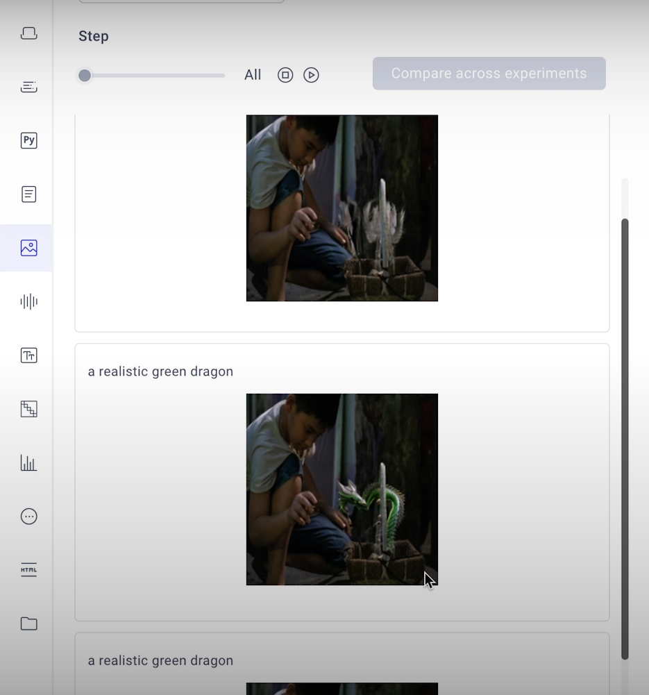
The strength hyperparameter is only used in image-to-image diffusion models. When we try to inpaint using diffusion models, we add a lot of noise; the amount of noise we add determines how much information is eliminated, and strength is the hyperparameter that controls this.
strength_values = [x for x in np.arange(0.1, 1.1, 0.2)]
exp = comet_ml.Experiment()

prompt = "a realistic green dragon"

num_inference_steps = 200 if torch.cuda.is_available() else 10

exp.log_parameters({
    "seed": seed,
})
for strength in strength_values:

    output = sd_pipe(
      image=image,
      mask_image=image_mask,
      prompt=prompt,
      generator=generator,
      num_inference_steps=num_inference_steps,
      strength=strength
    )

    generated_image = output.images[0]

    exp.log_image(
        generated_image,
        name=f"{prompt}",
        metadata={
            "prompt": prompt,
            "seed": seed,
            "num_inference_steps": num_inference_steps,
            "strength": strength
        }
    )

exp.end()

reference_experiment = comet_ml.APIExperiment(
    workspace="ckaiser",
    project_name="4-diffusion-prompting",
    previous_experiment="2964615a382d46f09c3a36c50c74deef"
)

reference_experiment.display(tab="images")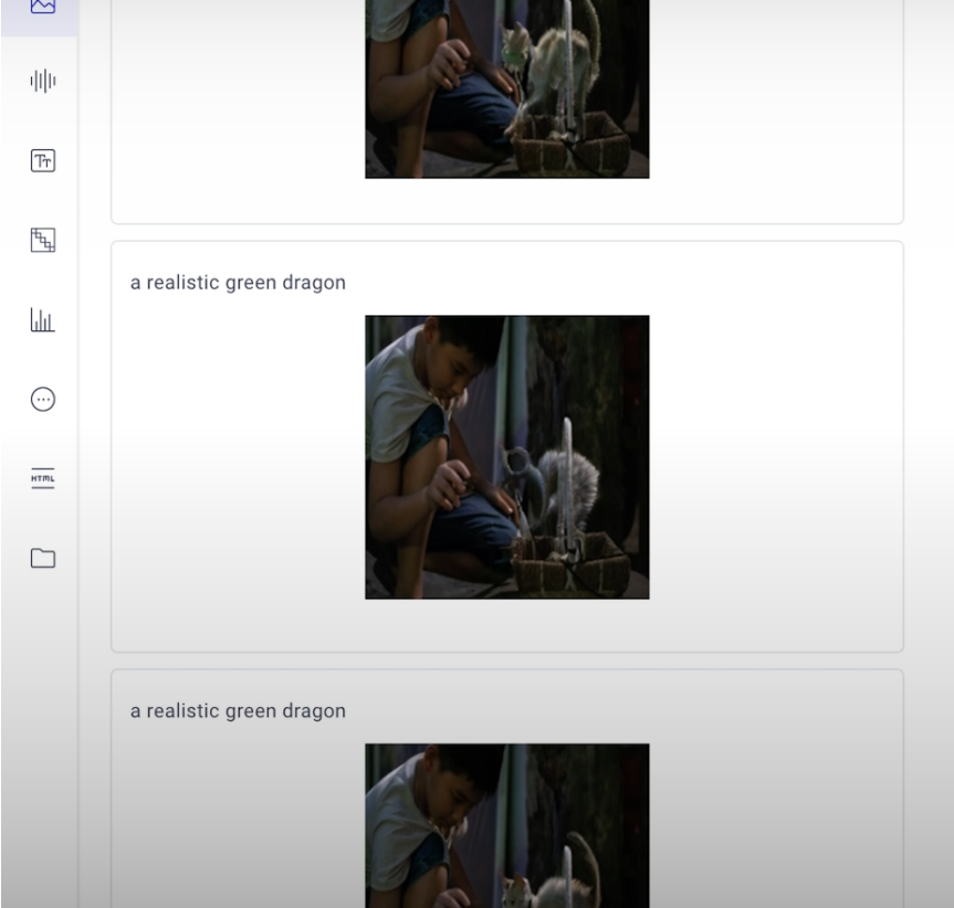
If you set the negative prompt to cartoon, the image creation model will not generate a picture that resembles a cartoon.
exp = comet_ml.Experiment()

prompt = "a realistic green dragon"
negative_prompt = "cartoon"

num_inference_steps = 100 if torch.cuda.is_available() else 10

exp.log_parameters({
    "seed": seed,
})
output = sd_pipe(
  image=image,
  mask_image=image_mask,
  prompt=prompt,
  negative_prompt=negative_prompt,
  generator=generator,
  num_inference_steps=num_inference_steps,
  guidance_scale=10
)

generated_image = output.images[0]

exp.log_image(
    generated_image,
    name=f"{prompt}",
    metadata={
        "prompt": prompt,
        "seed": seed,
        "num_inference_steps": num_inference_steps,
        "guidance_scale": 10
    }
)

exp.end()

reference_experiment = comet_ml.APIExperiment(
    workspace="ckaiser",
    project_name="4-diffusion-prompting",
    previous_experiment="f05b04ac203a4f9aa606ea6cf9417fa3"
)

reference_image = reference_experiment.get_asset_by_name(f"{prompt}")

plt.imshow(Image.open(io.BytesIO(reference_image)))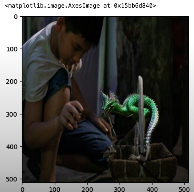
Additional Resources
- For more on how to use Comet [https://www.comet.com/site/?utm_source=dlai&utm_medium=course&utm_campaign=prompt_engineering_for_vision_models&utm_content=dlai_L4] for experiment tracking, check out Quickstart Guide [https://colab.research.google.com/drive/1jj9BgsFApkqnpPMLCHSDH-5MoL_bjvYq?usp=sharing] and the Comet Docs [https://www.comet.com/docs/v2/?utm_source=dlai&utm_medium=course&utm_campaign=prompt_engineering_for_vision_models&utm_content=dlai_L4].
- This course was based on a set of two blog articles from Comet. Explore them here for more on how to use newer versions of Stable Diffusion in this pipeline, additional tricks to improve your inpainting results, and a breakdown of the pipeline architecture:
- SAM + Stable Diffusion for Text-to-Image Inpainting: [https://www.comet.com/site/blog/sam-stable-diffusion-for-text-to-image-inpainting/?utm_source=dlai&utm_medium=course&utm_campaign=prompt_engineering_for_vision_models&utm_content=dlai_L4]
- Image Inpainting for SDXL 1.0 Base Model + Refiner: [https://www.comet.com/site/blog/image-inpainting-for-sdxl-1-0-base-refiner/?utm_source=dlai&utm_medium=course&utm_campaign=prompt_engineering_for_vision_models&utm_content=dlai_L4]
Finetuning
When prompt and hyperparameter tuning are insufficient, it is time to fine-tune. Finetuning is quite resource-heavy, but there is a method of finetuning stable diffusion that utilizes significantly fewer resources, known as Dreambooth.How could we train a model to visualize you as a Van Gogh painting? Dreambooth is intended to teach models new things with extremely small quantities of sample data.
Finetuning should be done with enough data to allow the model to generalize without compromising the model's performance on other tasks. For example, we can train our image model to produce our faces, but it may begin to produce everyone's faces as well.
DreamBooth addresses each of these issues in large part by exploiting the diffusion model's prior knowledge of the environment. The authors of DreamBooth refer to this as the Semantic Prior Knowledge. Consider using context hints when reading a new term. When the model encounters a cue, such as a photo of a man called Andrew, it may not know what Andrew looks like, but it does know how a man appears, and it uses this information in training, allowing us to train with a lot smaller example dataset.
First, you choose a token that the model rarely sees, such as this bracketed [V]. Your training loop will overwrite the data in the model associated with this token. This is comparable to many other methods for changing diffusion models you may come across. Then, you combine this unusual token with another token that broadly identifies the class to which your subject belongs.
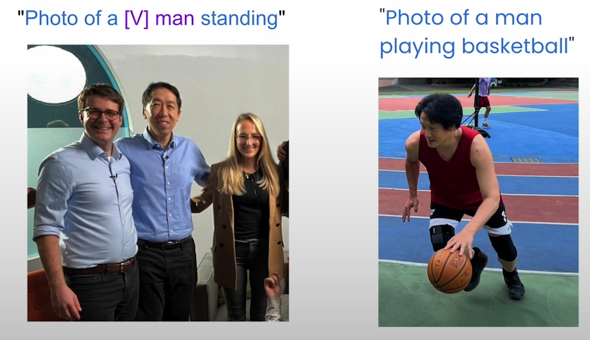
This does not resolve the language drift issue. The paper developed a bespoke loss metric called a previous preservation loss, which employs an intriguing type of regularization. Regularization penalizes the model for deviating from its initial knowledge when fine-tuning. You construct a series of image prompt pairs.
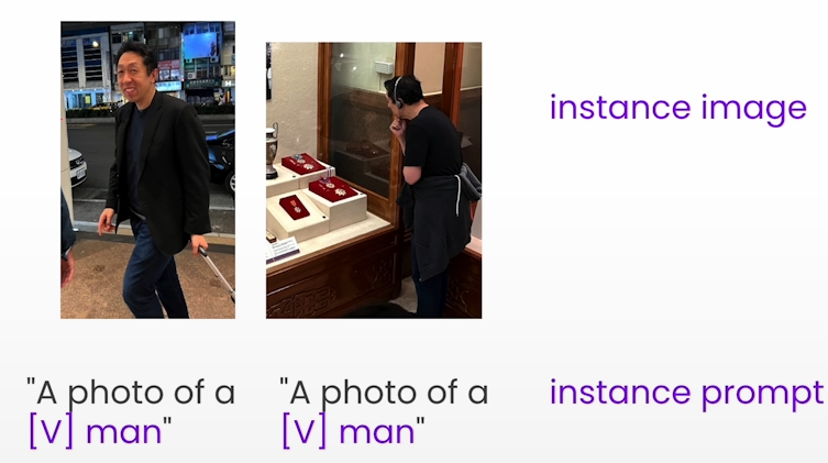
You can use BLIP: image captioning auto-generate instance prompts.
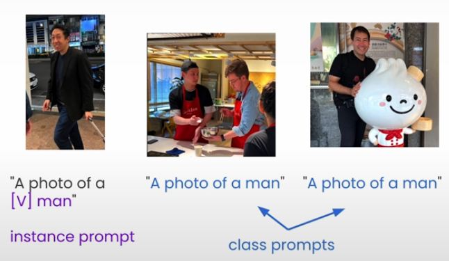
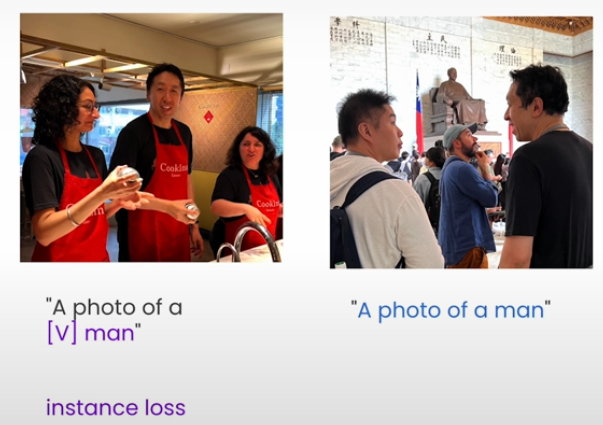
Now that we have 10 instance prompts, we need to construct 100 class prompts, which includes a photo of a man who is not Andrew. Using these photos, you may create a robust distribution that represents the model's past comprehension of the prompt concepts. During the training procedure, you will calculate two losses.
During the training procedure, you will calculate two losses. First, you calculate the loss using the instance data. It indicates how well the model reconstructs Andrew's visuals when given our changed token pair. Second, you compute the loss for the class dataset. In other words, how close does the model get to creating an image from the prior distribution when presented with the class prompt?
import comet_ml
comet_ml.login(anonymous=True)

# Import and prepare the model
import torch
if torch.cuda.is_available():
    model_name = 'stabilityai/stable-diffusion-xl-base-1.0'
else:
    model_name = './models/runwayml/stable-diffusion-v1-5'

# Define hyperparameters
"""
If you have GPU it will run Stable Diffusion XL, if you do not it will use version 1.5 on CPU
Different diffusion models perform better at different sizes thats why resolution is dynamic.
The prior loss weight is a numeric value that scales our class loss when we are calculating our prior preservation loss.
If we do not care about catastrophic forgetting we can set the prior loss weight to 0 else higher value.
"""
hyperparameters = {
    "instance_prompt": "a photo of a [V] man",
    "class_prompt": "a photo of a man",
    "seed": 4329,
    "pretrained_model_name_or_path": model_name,
    "resolution": 1024 if torch.cuda.is_available() else 512,
    "num_inference_steps": 50,
    "guidance_scale": 5.0,
    "num_class_images": 200,
    "prior_loss_weight": 1.0
}
experiment = comet_ml.Experiment()
# Load images
from utils import DreamBoothTrainer
trainer = DreamBoothTrainer(hyperparameters)

# Required GPU
# To run the training pipeline
trainer.generate_class_images()
# To see the content of generate_class_image
??trainer.generate_class_images

# Get class images using artifacts
import shutil
# Get images
class_artifact = experiment.get_artifact('ckaiser/class-images-15')
class_artifact.download('./')
shutil.unpack_archive('./class.zip', './class')

# Print some images
trainer.display_images("class")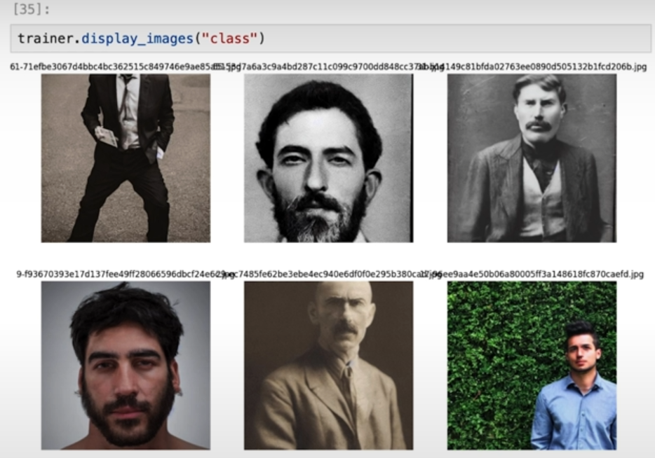
andrew_artifact = experiment.get_artifact('ckaiser/andrew-dataset')
andrew_artifact.download('./')
shutil.unpack_archive('./andrew-dataset.zip', './instance')
# Print some images
trainer.display_images("instance")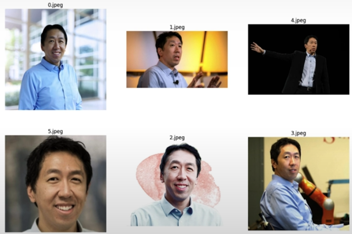
# Initialize the model (takes several minutes)
tokenizer, text_encoder, vae, unet = trainer.initialize_models()

# Add noise to generate images in Stable Diffusion
from diffusers import DDPMScheduler
noise_scheduler = DDPMScheduler.from_pretrained(
    trainer.hyperparameters.pretrained_model_name_or_path,
    subfolder="scheduler"
)
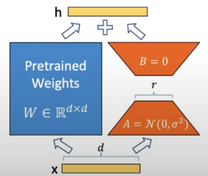
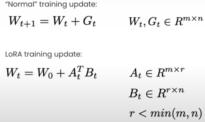
LoRA: Low-Rank Adaptation Tuning is a technique for fine-tuning models that involves training a small set of adapter weights. It takes advantage of the low intrinsic rank of update matrices during training. The article "LoRA: Low-Rank Adaption of Language Model by Hu et al" introduces it. To put it simply, instead of training the entire network, we add and train an adapter that represents 1% to 2% of the network.
unet = trainer.initialize_lora(unet)
optimizer, params_to_optimize = trainer.initialize_optimizer(unet)
# Initialize the datasets
train_dataset, train_dataloader = trainer.prepare_dataset(tokenizer, text_encoder)
lr_scheduler = trainer.initialize_scheduler(train_dataloader, optimizer)
unet, optimizer, train_dataloader, lr_scheduler = trainer.accelerator.prepare(
    unet, optimizer, train_dataloader, lr_scheduler)
total_batch_size = \
    trainer.hyperparameters.train_batch_size * \
    trainer.hyperparameters.gradient_accumulation_steps

# Requires GPU
from tqdm import tqdm

global_step = 0
epoch = 0

progress_bar = tqdm(
    range(0, trainer.hyperparameters.max_train_steps),
    desc="Steps"
)
for epoch in range(0, trainer.hyperparameters.num_train_epochs):
    unet.train()
    # Convert image to latent representation, pass pixel representation into variational auto encoder and sample from latent distribution
    # Once we converted our image into its latent representation, we sample the noise that we are going to add to the latents as we train
    # We need to add our noise to random timesteps, after diffusion is done we need to do reverse diffusion
    # To do reverse diffusion we need to get embeddings of our prompt and use U-Net model to predict the noise in the image.
    # Once our loss have been calculated we can perform backpropagation and step our optimizer as you would in any other training loop
    for step, batch in enumerate(train_dataloader):
        with trainer.accelerator.accumulate(unet):
            pixel_values = batch["pixel_values"].to(dtype=vae.dtype)
            model_input = vae.encode(pixel_values).latent_dist.sample()
            model_input = model_input * vae.config.scaling_factor

            noise = torch.randn_like(model_input)
            bsz, channels, height, width = model_input.shape

            timesteps = torch.randint(
                0,
                noise_scheduler.config.num_train_timesteps,
                (bsz,),
                device=model_input.device
            )

            timesteps = timesteps.long()
            noisy_model_input = noise_scheduler.add_noise(
                model_input,
                noise,
                timesteps
            )

            encoder_hidden_states = batch["input_ids"]

            model_predict = unet(
                noisy_model_input,
                timesteps,
                encoder_hidden_states,
                return_dict=False,
            )[0]

            target = noise

            model_pred, model_pred_prior = torch.chunk(model_pred, 2, dim=0)
            target, target_prior = torch.chunk(target, 2, dim=0)

            instance_loss = \
                F.mse_loss(
                    model_pred.float(),
                    target.float(),
                    reduction="mean"
                )

            prior_loss = \
                F.mse_loss(
                    model_pred_prior.float(),
                    target_prior.float(),
                    reduction="mean"
                )

            loss = \
                instance_loss + \
                trainer.hyperparameters.prior_loss_weight * \
                prior_loss

            trainer.accelerator.backward(loss)
            optimizer.step()
            lr_scheduler.step()
            optimizer.zero_grad()
            global_step +=1

        loss_metrics = {
            "loss": loss.detach().item,
            "prior_loss": prior_loss.detach().item,
            "lr": lr_scheduler.get_last_lr()[0],
        }

        experiment.log_metrics(loss_metrics, step=global_step)

        progress_bar.set_postfix(**loss_metrics)
        progress_bar.update(1)

        if global_step >= trainer.hyperparameters.max_train_steps:
            break

    trainer.save_lora_weights(unet)
experiment.add_tag(f"dreambooth-training")
experiment.log_parameteres(trainer.hyperparameters)
trainer.accelerator.end_training()

# Retrieve the training results
training_experiment = \
    comet_ml.APIExperiment(
        previous_experiment="d92519b1f657497e8569a2c8e989b457"
    )
# See the experiment
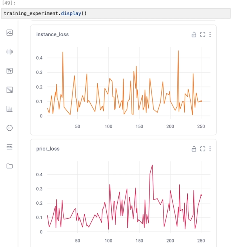
training_experiment.display()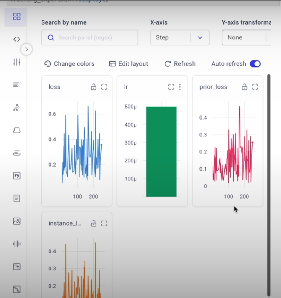
Throughout this course, we've stressed the significance of working with your picture data and visually inspecting your model's results. You can observe that the loss appears to overcorrect back and forth between the previous loss and the instance loss. Peaks in the past loss typically correspond to valleys in the instance loss, and vice versa.
# Prompts to generate images of Andrew
prompts = [
    "a photo of a [V] man playing basketball",
    "a photo of a [V] man riding a horse",
    "a photo of a [V] man at the summit of a mountain",
    "a photo of a [V] man driving a convertible",
    "a photo of a [V] man riding a skateboard on a huge halfpipe",
    "a mural of a [V] man, painted by graffiti artists"
]

validation_prompts = [
    "a photo of a man playing basketball",
    "a photo of a man riding a horse",
    "a photo of a man at the summit of a mountain",
    "a photo of a man driving a convertible",
    "a photo of a man riding a skateboard on a huge halfpipe",
    "a mural of a man, painted by graffiti artists"
]

# Following code requires GPU
from diffusers import DiffusionPipeline
pipeline = DiffusionPipeline.from_pretrained("runwayml/stable-diffusion-v1-5")
pipeline.load_lora_weights("./andrew-model")
for prompt in prompts:
    with torch.no_grad():
        images = pipeline(
            prompt = prompt,
        ).images

        experiment.log_image(images[0], metadata={
            "prompt": prompt,
            "model": hyperparameters.pretrained_model_name_or_path,
        })
for prompt in validation_prompts:
    with torch.no_grad():
        images = pipeline(
            prompt=prompt,
        ).images

    experiment.log_image(images[0], metadata={
            "prompt": prompt,
            "model": hyperparameters.pretrained_model_name_or_path,
        })

# Retrieve the image generation results (You can view the results of image generation regardless of whether you have access to GPUs, using the experiment tracking tool.)
inference_experiment = comet_ml.APIExperiment(
        previous_experiment="0eb292126ab5476ab0c863061a400bdc"
    )
# See the experiment
inference_experiment.display(tab="images")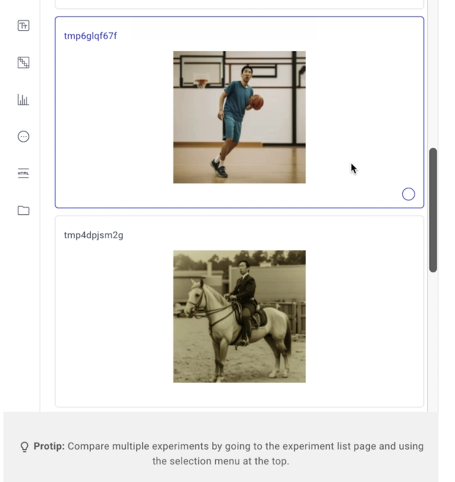
Additional Resources
- For more on how to use Comet for experiment tracking, check out this Quickstart Guide and the Comet Docs.
- This course was based on a set of two blog articles from Comet. Explore them here for more on how to use newer versions of Stable Diffusion in this pipeline, additional tricks to improve your inpainting results, and a breakdown of the pipeline architecture:
- SAM + Stable Diffusion for Text-to-Image Inpainting: [https://www.comet.com/site/blog/sam-stable-diffusion-for-text-to-image-inpainting/?utm_source=dlai&utm_medium=course&utm_campaign=prompt_engineering_for_vision_models&utm_content=dlai_L5]
- Image Inpainting for SDXL 1.0 Base Model + Refiner: [https://www.comet.com/site/blog/image-inpainting-for-sdxl-1-0-base-refiner/?utm_source=dlai&utm_medium=course&utm_campaign=prompt_engineering_for_vision_models&utm_content=dlai_L5]
Resources
[1] Deeplearning.ai, (2024), Prompt Engineering for Vision Models:
[https://www.deeplearning.ai/short-courses/prompt-engineering-for-vision-models/]


0 Comments