
https://medium.com/@cbarkinozer/pytorch-ustal%C4%B1k-serisi-b%C3%B6l%C3%BCm-2-036c30c47b8b
Part 2 in a series I started to provide a detailed tutorial on building and training neural networks with PyTorch.

Reshaping Viewing, Stacking and Squeezing Tensors
Pytorch's most prevalent problems are shape-related, and reshaping is the most common action used to address them.
The view returns a view of a tensor of a specific shape while maintaining the same memory as the original tensor. Shaping and viewing are generally equivalent, although view always retains the same memory as the original tensor.
Stacking is the process of arranging numerous tensors on top of one another (vstack) or side by side (hstack).
Squeeze eliminates one dimension from a tensor. Unsqueeze adds one dimension to the target tensor.
Permute returns a view of an input with its dimensions permuted (swapped) in a certain way. In simpler terms, you can rearrange items in the desired order.
import pytorch

x = torch.arange(1.,10.)
print(x) # tensor([1., 2., 3., 4., 5., 6., 7., 8., 9.])
print(x.shape) # torch.Size([9])

# Add an extra dimension
x_reshaped = x.reshape(1,9)

# Change the view
z = x.view(1,9)

# x_reshaped and z variables are same but z will point the same memory point as x
# So changing z changes x

x_stacked = torch.stack([x,x,x,x], dim=0) # Works
x_stacked = torch.stack([x,x,x,x], dim=1) # Works
x_stacked = torch.stack([x,x,x,x], dim=2) # NOT VALID


x = torch.zeros(2, 1, 2, 1, 2)
x.size() # torch.Size([2, 1, 2, 1, 2])

y = torch.squeeze(x)
y.size() # torch.Size([2, 2, 2])

y = torch.squeeze(x, 0)
y.size() # torch.Size([2, 1, 2, 1, 2])

y = torch.squeeze(x, 1)
y.size() # torch.Size([2, 2, 1, 2])

y = torch.squeeze(x, (1, 2, 3)) # torch.Size([2, 2, 2])

x = torch.tensor([1, 2, 3, 4])
torch.unsqueeze(x, 0) # tensor([[ 1,  2,  3,  4]])

torch.unsqueeze(x, 1)
# tensor([[1],[2],[3],[4]])


x = torch.randn(2, 3, 5)
x.size() # torch.Size([2, 3, 5])
torch.permute(x, (2, 0, 1)).size() # torch.Size([5, 2, 3])
Selecting data from tensors
Indexing using Pytorch is comparable to indexing with NumPy.
import torch

x = torch.arange(1,10).reshape(1,3,3)
print(x)
'''
tensor([[[1, 2, 3],
         [4, 5, 6],
         [7, 8, 9]]])
'''
print(x.shape) # torch.Size([1, 3, 3])
Let's index our new tensor.
print(x[0])
'''
tensor([[[1, 2, 3],
         [4, 5, 6],
         [7, 8, 9]]])
'''
Let's start by indexing the center array, which represents the first dimension.
print(x[0][0]) # tensor([1, 2, 3])
print(x[0, 0]) # tensor([1, 2, 3])
print(x[:,0])  # tensor([1, 2, 3])
print(x[0,0,:])# tensor([1, 2, 3])
print(x[0][1][1]) # tensor(5)
Pytorch and Numpy
Because NumPy is a scientific Python numerical computing package, Pytorch may interface with it.
import numpy as np

array = np.arange(1.0, 8.0)
tensor = torch.from_numpy(array)
print(array) # [1. 2. 3. 4. 5. 6. 7.]
print(tensor) # tensor([1., 2., 3., 4., 5., 6., 7.], dtype=torch.float64)
In NumPy, the default type is float64, however this can be changed.
tensor32 = tensor.type(float32)Pytorch Reproducibility (taking out random out of random)
How does a neural network learn?
start with random numbers -> tensor operations -> update random numbers to try to make them better representations of the data -> Repeat
When you desire reproducibility, you don't want too much unpredictability.
torch.rand(3,3)To reduce unpredictability, there is a notion known as random seed. True randomness is not possible in computer science. You receive pseudo-randomness, often known as produced randomness. For example, in computer science, the exact year, month, day, minute, and second are used as seeds for some algorithms. Some scientists recommend employing cosmic radiations, for example, to achieve the best unpredictability possible.
import torch

RANDOM_SEED = 42
torch.manual_seed(RANDOM_SEED)
random_tensor_c = torch.rand(3,4)

torch.manual_seed(RANDOM_SEED)
random_tensor_d = torch.rand(3,4)

print(random_tensor_c == random_tensor_d)
Accessing a GPU
You need a GPU to do larger tensor operations faster thanks to CUDA. A GPU can be accessed for free through Google Collab, by purchasing GPU hardware, or through cloud computing services like as AWS and Azure.
Run the following to check for GPU in Google Collab:
import torch
torch.cuda.is_available()
Run the following command to check for an Nvidia GPU after downloading CUDA to your local or cloud device:
nvidia-smiTo set device agnostic code:
device = "cuda" if torch.cuda.is_available() else "cpu"To count the number of devices:
torch.cuda.device_count()When we create a tensor, it will operate on CPU by default; however, we want to run on GPU because it is much faster:
tensor = torch.tensor([1,2,3])

print(tensor.device) # cpu

device = "cuda" if torch.cuda.is_available() else "cpu"
tensor_on_gpu = tensor.to(device)
print(tensor_on_gpu.device) # cuda:0
Below is an example of the most popular 3rd type of error in Pytorch, the device error.
tensor_on_gpu.numpy() # Can't convert cuda:0 device type tensor to numpy.
#Use Tensor.cpu() to copy the tensor to host memory first.
To fix the GPU tensor with the NumPy issue, we can first set it to the CPU
tensor_on_gpu.cpu().gpu()Congratulations this is the end of the Pytorch Fundamentals. For more check exercises and extra curriculum: https://www.learnpytorch.io/00_pytorch_fundamentals/#exercises
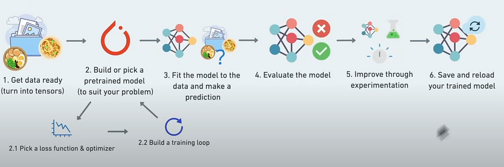
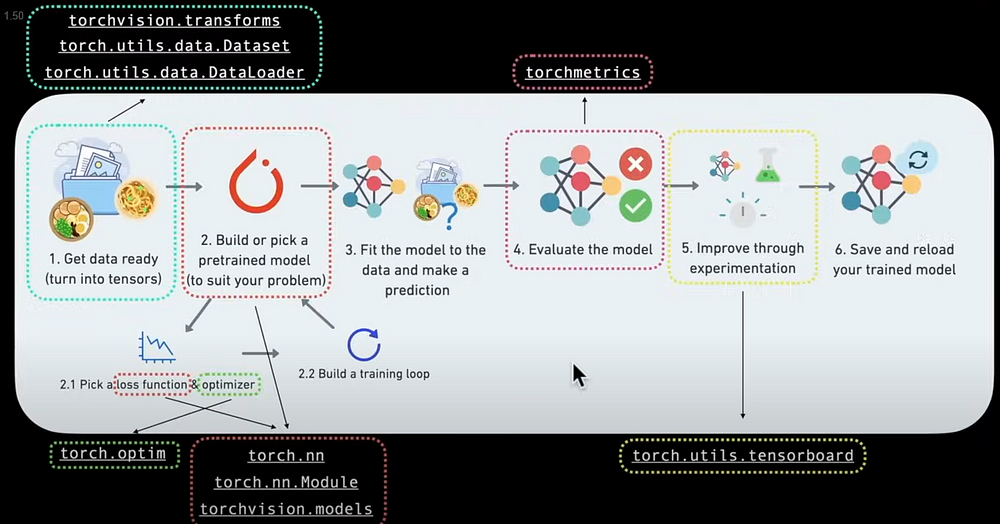
Pytorch Workflow
nn contains all of Pytorch's building blocks for neural networks:
from torch import nnCheck Pytorch version:
torch.__version__Data Preparing and Loading
Data can be anything, including excel spreadsheets, photos, movies, music, DNA, and text.
Fundamentally, data preparation entails converting data into a numerical representation, while loading entails creating a model that learns patterns in that numerical representation.
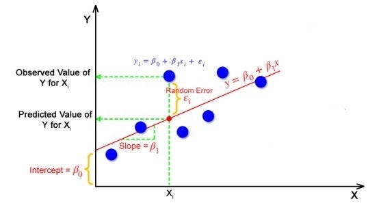
Let's start with the most fundamental model in machine learning: linear regression. The linear regression formula is: y = weight * X + bias. This model creates a straight line between data points.
weight = 0.7
bias = 0.3

start = 0
end = 1
step = 0.02
X = torch.arange(start, end, step).unsqueeze(dim=1)
y = weight * X + bias
print(len(X)) # 50
print(len(y)) # 50
The X is capitalized because capital letters represent matrices and tensors, whereas small letters represent vectors.
Generalization refers to a machine learning model's capacity to perform effectively on new data.
Datasets typically consist of three parts: training (60-80%), testing (10-20%), and validation (10-20%). While train and test sets are always present, validation datasets are frequently but not always available.
The model learns from the training data.
Validation Data: The model is tweaked using this data (similar to the practice exam you take before the final exam).
Test Data: This data is used to evaluate the model's learning (similar to the final exam at the end of the semester).
Create a test-train split:
train_split = int(0.8 * len(X))
X_train, y_train = X[:train_split], y[:train_split]
X_test, y_test = X[train_split], y[train_split]
When you use sklearn.train_test_split, it adds a small amount of randomization while dividing.
def plot_predictions(train_data=X_train,
 train_labels=y_train,
 test_data=X_test,
 test_labels=y_test,
 predictions=None):
  """Plots training data, test data and compares predictions."""
  plt.figure(figsize=(10, 7))

  # Plot training data in blue
  plt.scatter(train_data, train_labels, c="b", s=4, label="Training data")

  # Plot test data in green
  plt.scatter(test_data, test_labels, c="g", s=4, label="Testing data")

  # Are there predictions?
  if predictions is not None:
    # Plot the predictions if they exist
    plt.scatter(test_data, predictions, c="r", s=4, label="Predictions")

  # Show the legend
  plt.legend(prop={"size": 14})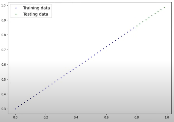
Building a Model in Pytorch
Almost everything in Pytorch inherits nn.Module .
from torch import nn

class LinearRegressionModel(nn.Module):
  def __init__(self):
    super().__init__()
    self.weights = nn.Parameter(torch.randn(1, requires_grad=True,dtype=torch.float))
    self.bias = nn.Parameter(torch.randn(1, requires_grad=True,dtype=torch.float))
    # Forward  method to define the computation in the model
    def forward(self, x: torch.Tensor) -> Torch.tensor:
      return self.weights * x + self.bias # linear regression
This code begins with random weights and biases, then examines random data and adjusts the weights and biases as closely to the data as possible.
How does the model change its weights and biases?
Using gradient descent and backpropagation.
Below are some excellent animated explanation videos that answer three basic questions. You can watch them. The videos are in English, but with Turkish subtitles.
What is gradient descent?
Gradient descent is an optimization approach that is widely utilized in machine learning and mathematical optimization. Its primary goal is to minimize a function by iteratively traveling in the direction of the function's steepest fall (negative gradient).
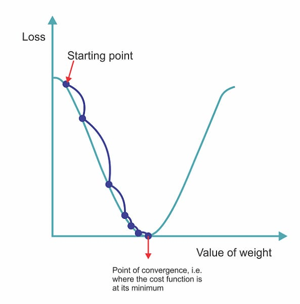
- Initialization: Make an initial guess for the parameters of the function being optimized. These parameters are sometimes abbreviated as theta (θ).
- Calculate Gradient: Calculate the gradient of the goal function in terms of the parameters. The gradient indicates the direction of the steepest ascent. In other words, it represents the direction in which the function increases the most rapidly.
- Update parameters: To minimize the objective function, move the parameters in the opposite direction as the gradient. This is accomplished by removing a portion of the gradient (scaled by the learning rate) from the current parameter values. The formula for updating parameters is: θ=θ−α∇J(θ), where:
- θ represents the parameters being optimized.
- α (alpha) is the learning rate, a small positive scalar that determines the step size.
- ∇J(θ) denotes the gradient of the objective function J(θ) with respect to θ.
4. Iterate: Repeat steps 2 and 3 until a stopping point is reached. This criterion could include a maximum number of iterations, achieving a specified level of convergence, or other conditions unique to the issue being solved.
The algorithm iteratively modifies the parameters to minimize the objective function, gradually converging to a local minimum (or, in certain situations, a global minimum). The learning rate is a vital hyperparameter that must be carefully selected, as a low value may result in slow convergence, whereas a high number may lead the algorithm to diverge or fluctuate around the minimum.
How does backpropagation work?
Check the 3 brown 1 blue Youtube channels video about this topic.
torch.nn: Includes all of the buildings for computational graphs (neural networks).
torch.nn.Parameter: What parameters should our model aim to learn, such as a Pytorch layer from Torch.nn will set it for us.
torch.nn.Module: The base class for all neural network modules. If you subclass it, you must override it.
torch.optim: This is where Pytorch's optimizers dwell; they assist with gradient descent.
def forward(): All nn.Module subclasses require you to overwrite forward(), which describes what happens during forward computation.
torch.utils.data.Dataset: Represents a map of your data's key (label) and sample (feature) pairs. As an example, consider photos and their labels.
torch.utils.data.Dataloader: Creates a Python iterable over a torch dataset (which allows you to iterate over the data).
For more, check Pytorch cheatsheat: https://pytorch.org/tutorials/beginner/ptcheat.html
Let's see what's inside our model:
torch.manuel_seed(42)

model_0 = LinearRegressionModel()

print(list(model_0.parameters())
# [tensor([[-0.1234], ...]),  # Weights tensor (example values shown)
# tensor([0.0])]  # Biases tensor (example values shown)
print(model_0.state_dict()) # OrderedDict([('weights',tensor([0.3367])),('bias',tensor([0.1288]))])
Making Predictions
Let's evaluate our model's prediction power.
torch.no_grad():
Pytorch provides a context manager. When enabled, PyTorch disables gradient calculation for all actions performed within this context. This implies that no gradients will be computed for the tensors involved in those operations. This is generally used in inference or validation when gradients are not required and you want to speed up computations by not keeping intermediate values for backward passes.
torch.inference_mode():
It is intended to optimize computation for inference purposes, such as lowering memory footprint and maybe enabling additional optimizations. When enabled, it may alter the behavior of specific processes to increase inference performance. Unlike torch.no_grad(), torch.inference_mode() affects not only gradient computation but also how operations are done. This method is mostly used for installing PyTorch models in production contexts where inference speed and resource utilization are crucial.
with torch.inference_mode():
  y_preds1 = model_0(X_test)

with torch.no_grad():
  y_preds2 = model_0(X_test)

print(y_preds1)
print(y_preds2)
print(y_test)
# Both results are far away from close but not hallicunations (too irrelevant)
plot_predictions(predictions=y_preds1)
plot_predictions(predictions=y_preds2)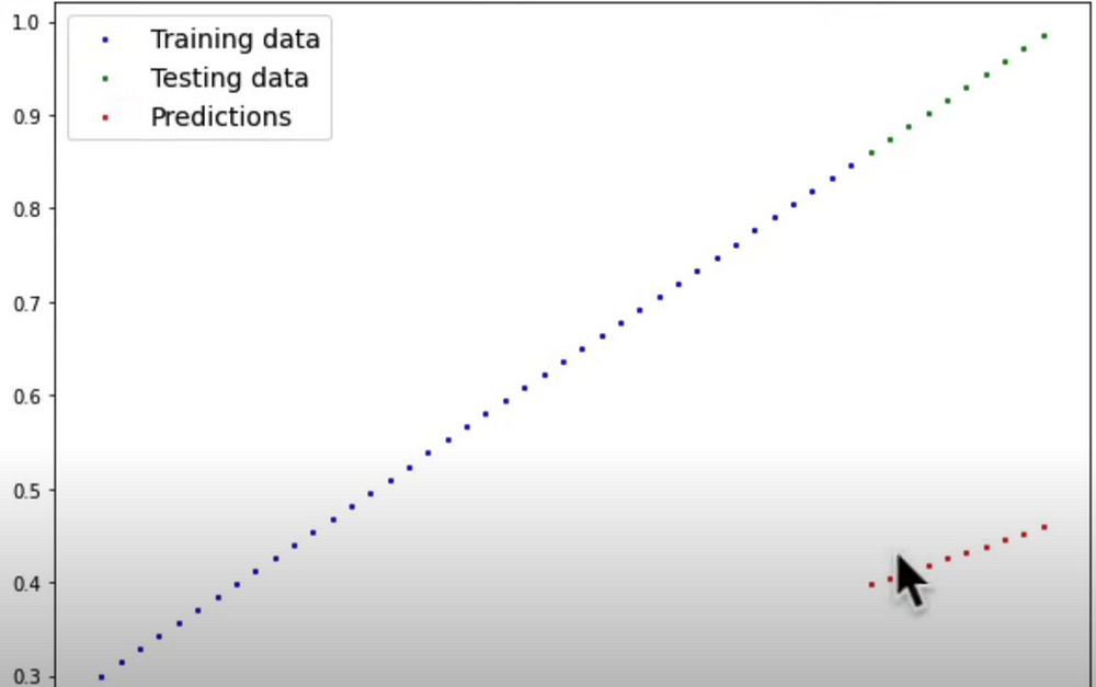
The training is intended to produce a model that describes the relationship/pattern in the data.
A loss function can be used to assess the success of the model's summary ability. In several contexts, the loss function is referred to as a cost function or criterion.
All loss functions are available in torch.nn: https://pytorch.org/docs/stable/nn.html#loss-functions
An optimizer evaluates the loss function findings and adjusts the model's parameters.
Mean Absolute Error (MAE)
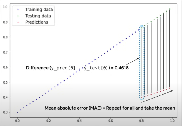
MAE is a popular loss function. MAE calculates the mean of the difference between the predicted and actual values. Can be used as follows:
MAE_loss =  torch.nn.L1Loss

# stochastic gradient descend as optimizer (lr= learning rate)
optimizer = torch.optim.SGD(params=model.parameters(), lr=0.001)
The loss function and optimizer you should employ are problem-specific. For example, for a linear regression model, L1Loss as the loss function and SGD as the optimizer will suffice. For a classification task, the loss function nn.BCELoss() (Binary Cross Entropy Loss) and the optimizer torch.optim.RMSProp() will suffice.
Building a training and testing loop in Pytorch
- Loop through the data.
- To make predictions on propagations, we use the forward() function to transmit input through our model's parameters.
- Calculate Loss
- Optimizer zero grad
- Move backwards through the network to calculate the gradients of each parameter on the loss.
- Optimizer/gradient descent (use optimizer to alter model parameters to try to improve loss)
An epoch is a single loop over the data.
Hyperparameters are variables that people fine-tune to ensure the model operates optimally. There are no perfect right values, thus people fine-tune them.
epochs = 1

for epoch in range(epochs):
  model_0.train()
  y_pred = model_0(X_train)
  loss= loss_fn(y_pred, y_train)
  optimizer.zero_grad()
  loss.backward()
  optimizer.step()
  model_0.eval() # turns of gradient tracking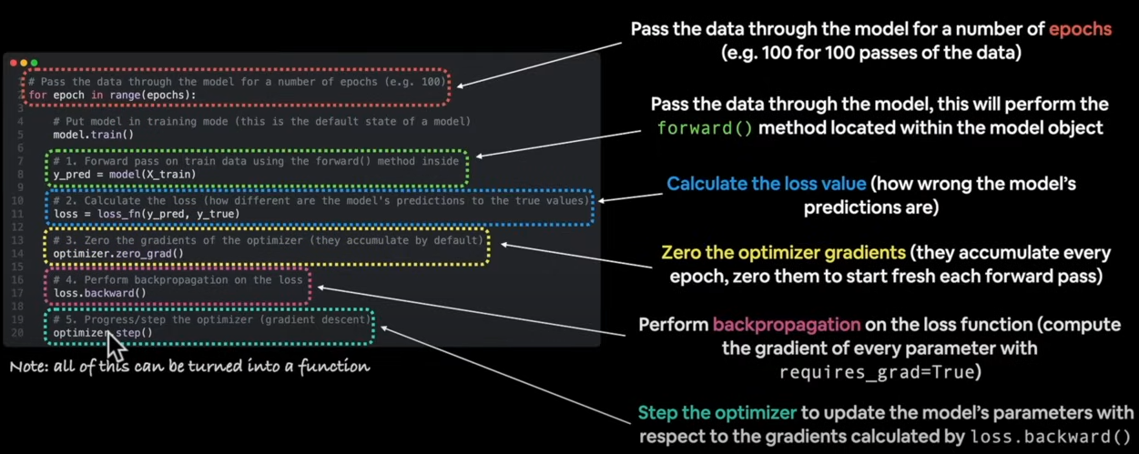
Let’s run our model
epochs = 100

for epoch in range(epochs):
  model_0.train()
  y_pred = model_0(X_train)
  loss = loss_fn(y_pred, y_train)
  optimizer.zero_grad()
  loss.backward()
  optimizer.step()
  model_0.eval()

with torch.inference_mode():
  y_preds_new = model_0(X_test)

plot_predictions(predictions= y_preds_new)
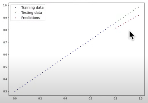
The figure above shows that the predictions are becoming more accurate. If we run another 100 epochs, the model will get closer, but there is a chance that the model will memorize that data, thus we would like not get closer than 95%.
The final step is to save the model once we've finished constructing it.
Saving the Model
There are several methods for saving and loading models in Pytorch. You can save and load the state_dict or the entire model. A state_dict is essentially a Python dictionary object that maps each layer to the corresponding parameter tensor. The model's state_dict only contains entries for layers with learnable parameters (convolutional layers, linear layers, etc.) and registered buffers (batchnorm's running_mean).
- torch.save(): Allows you to save a Pytorch object in Python’s pickle format.
- torch.load(): Allows you to load a saved Pytorch object.
- torch.nn.Module.load_state_dict(): This allows to load a model’s saved state dictionary.
from pathlib import Path

MODEL_PATH = Paths("models")
MODEL_PATH.mkdir(parents=True, exist_ok=True)

MODEL_NAME="01_pytorch_workflow_model_0.pth"
MODEL_SAVE_PATH= MODEL_PATH/ MODEL_NAME

# saving the model
torch.save(obj=model_0.state_dict(), f=MODEL_SAVE_PATH)
# loading the model
loaded_model = LinearRegressionModel().load_state_dict(torch.load(f=MODEL_SAVE_PATH))
Resource
[1] freeCodeCamp.org, (6 Ekim 2022), PyTorch for Deep Learning & Machine Learning — Full Course:


0 Comments