
The final episode of the series. We will create a food products application using our own data.
To work on our own models, we need to use custom datasets. To deal with our own bespoke datasets, we must first preprocess the data.
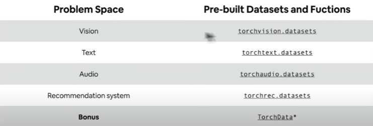
Pytorch Domain Libraries

Pytorch contains four primary domain libraries. TorchVision, TorchText, TorchAudio, and TorchRec (recommendations). TorchData also provides a variety of data loading helper functions.
We will create a tiny food classification software that will be educated using our custom photographs. The designer of this course also built the https://nutrify.app/, which categorizes and displays calories and health scores for various foods.
For this goal, we will do these:
- Obtaining a custom dataset with Pytorch.
Become one with the data by preparing and visualizing it.
Transforming data for use in a model.
Leading custom data using both pre-built and custom functions.
Creating FoodVision Mini to categorize food photos.
comparing models with and without data augmentation.
Making forecasts based on custom data.
Import Pytorch and build up device-agnostic code.
import torch
from torch import nn

print("Pytorch Version: "torch.__version__) # At least 1.10.0+ needed for this

device = "cuda" if torch.cuda.is_available() else "cpu"
print("Device: ",device)
Getting the dataset
Our dataset is a subset of the Food 101 dataset. Food101 launches 101 different food classes, each with 1000 photos (750 for training and 250 for testing). Our dataset starts with three food classes and only 10% of the photos (about 75 training and 25 testing). When launching ML initiatives, it's vital to start small and then grow up as needed. The main goal is to increase the pace at which you can experiment.
import requests
import zipfile
import pathlib import Path

# Setup path to a data folder
data_path = Path("data/")
image_path = data_path / "pizza_steak_sushi"

# If the image folder does not exist, download it and prepare it...
if image_path.is_dir():
  print(f"{image_path} directory already exists... skipping download")
else:
  print(f"{image_path} does not exist, creating one...")
  image_path.mkdir(parents=True, exist_ok=True)

# Download pizza, steak and sushi data
with open(data_path / "pizza_steak_sushi.zip", "wb") as f:
  request = request.get("https://github.com/mrdbourke/pytorch-deep-learning/raw/main/data/pizza_steak_sushi.zip")
  print("Downloading pizza, steak, sushi data...")
  f.write(request.content)

# Unzip pizza, steak, sushi data
with zipfile.ZipFile(data_path / "pizza_steak_sushi.zip", "r") as zip_ref:
  print("Unzipping pizza, steak and sushi data...")
  zip_ref.extractall(image_path)
Let’s become one with the data (data preparation and data exploration)
import os
def walk_through_dir(dir_path):
"""Walks through dir_path returning its contents."""
  for dirpath, dirnames, filenames in os.walk(dir_path):
    print(f"There are {len(dirnames)} directories and {len(filenames)} images in '{dirnames}'.")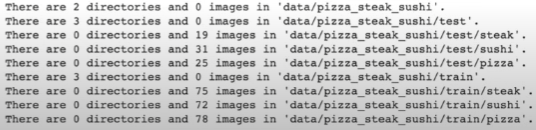
train_dir = image_path / "train"
test_dir = image_path / "test"

print(train_dir)
print(test_dir)
Visualizing an image
Let's write some code for:
Get all the picture paths.
Choose a random picture path with Python's random.choice().
'pathlib.Path.parent.stem' returns the image class name.
Since we're working with images, let's open them with Python's PIL.
We'll then display the image and output its metadata.
import random
from PIL import Image

random.seed(42)

# Get all image paths
image_path_list = list(image_path.glob("*/*/*.jpg"))

random_image_path = random.choice(image_path_list)

# Get image class from path name
image_class = random_image_path.parent.stem

img = Image.open(random_image_path)

print(f"Random image path: {random_image_path}")
print(f"Image class: {image_class}")
print(f"Image height: {img.height}")
print(f"Image width: {img.width}")
img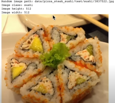
import numpy as np
import matplotlib.pyplot as plt

img_as_array = np.asarray(img)

plt.figure(figsize=(10,7))
plt.imshow(img_as_array)
plt.title(f"Image class: {image_class} | Image shape: {img_as_array_shape} -> [height, width, color_channels]")
plt.axis(False)
Transforming Our Data
Before we can use our image data in PyTorch:
Convert your target data into tensors (a numerical representation of our photos).
Create a 'torch.utils.data.Dataset' and then a 'torch.utils.data.DataLoader', which we'll refer to as 'Dataset' and 'DataLoader', respectively.
import torch
from torch.utils.data import DataLoader
from torchvision import datasets, transforms
Transforming data with torchvision.transforms
Transforms assist you prepare your photos for use with a model/perform data augmentation.
# Write a transform for image
data_transform = transforms.Compose([
  # Resize our images to 64x64
  transforms.Resize(size=(64x64))
  # Flip the images randomly on the horizontal
  transforms.RandomHorizontalFlip(p=0.5),
  # Turn the image into a torch.Tensor
  transforms.ToTensor()
])

data_transform(img)
def plot_transformed_images(image_paths, transform, n=3, seed=42):
"""Selects random iamges and loads/ trenasforms and then plots the original vs the transformed version."""
if seed:
random.seed(seed)
random_image_paths = random.sample(image_paths, k=n)
for image_path in random_image_paths:
with Image.open(image_path) as f:
fig, ax = plt.subplots(nrows=1, ncols=2)
ax[0].imshow(f)
ax[0].set_title(f"Original\nSize: {f.size}")
ax[0].axis(False)
# Transform and plot target image
transformed_image = transform(f).permute(1, 2, 0) # (C, H, W) -> (H, W, C)
ax[1].imshow(transformed_image)
ax[1].set_title(f"Transformed\nShape:" {transformed_image.shape})
ax[1].axis("off")
fig.suptitle(f"Class: {image_path.parent.stem}", fontsize=16)
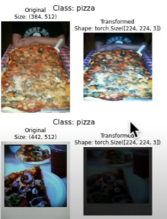
plot_transformed_images(image_paths=image_path_lsit, transform=data_transform, n=3, seed=42)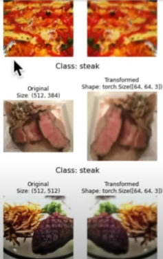
We reduced the amount of information so that we could work with performance, but we sacrificed accuracy.
Loading image data via 'ImageFolder'
Image categorization data can be loaded using 'torchvision.datasets.ImageFolder'.
# Use ImageFolder to create dataset(s)
from torchvision import datasets
train_data = datasets.ImageFolder(root=train_dir,
                                  transform=data_transform,
                                  target_transform=None)

test_data = datasets.ImageFolder(root=test_dir,
                                 transform=data_transform)

print(train_data)
print(test_data)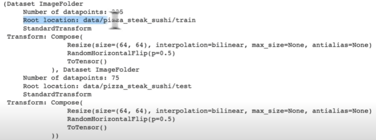
class_dict = train_data.class_to_idx
print(class_dict)
print(len(train_data))
print(len(test_data))

img, label = train_data[0][0], train_data[0][1]
print(f"Image tensor:\n {img}")
print(f"Image shape:\n {img.shape}")
print(f"Image datatype:\n {img.dtype}")
print(f"Image label:\n {label}")
print(f"Labeldatatype:\n {type(label)}")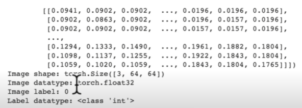
# Rearrange the order dimensions
img_permute = img.permute(1, 2, 0)

# Print out different shapes
print(f"Original shape: {img.shape} -> [color_channels, height, width]")
print(f"Image permute: {img_permute.shape} -> [height, width, color_channels]")

# Plot the image
plt.figure(figsize=(10,7))
plt.imshow(img_permute)
plt.axis("off")
plt.title(class_names[label], fontsize=14)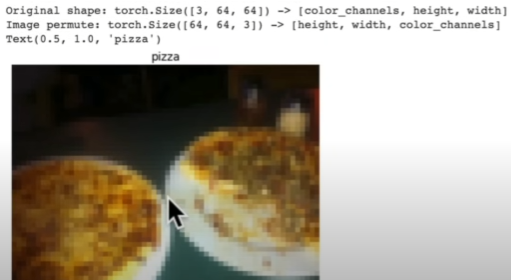
Turning loaded images into ‘DataLoader’s
A 'DataLoader' will assist us in converting our 'Dataset's' into iterables, and we can customize the batch_size so that our model may see batch_Size images at a time.
!nvidia-smi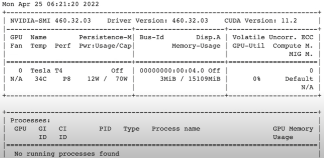
import os
os.cpu_count() # Check your machines cpu count.
# Turn train and test datasets into DataLoader's
from torch.utils.data import DataLoader
BATCH_SIZE=32
train_dataloader = DataLoader(dataset=train_dataset,
batch_size=BATCH_SIZE,
num_workers=1,
shuffle=True)
test_Dataloader = DataLoader(dataset=test_data,
batch_size=BATCH_SIZE,
num_workers=1,
shuffle=False)
print(len(train_dataloader)) # 8
print(len(test_dataloader)) # 3
print(len(train_data)) # 225
print(len(test_data)) # 75
len(train_data) / BATCH_SIZE ~= len(train_dataloader)
len(test_data) / BATCH_SIZE ~= len(test_dataloader)
img, label = next(iter(train_dataloader))

print(f"Image shape: {img.shape} -> [batch_size, color_channels, height, width]")
print(f"Label shape: {label.shape}")
Option: Loading Image Data with a Custom ‘Dataset’
- Able to load photos from a file.
Be able to extract class names from the dataset - Pros: Obtain classes as a dictionary from the dataset.
-
Can construct a 'dataset' from nearly anything.
Not restricted to Pytorch's pre-built 'Dataset' functions - Cons:
Creating a 'Dataset' from anything does not guarantee its functionality.
Using a custom 'Dataset' often requires us to write extra code, which might lead to errors or performance concerns. Pytorch libraries are extensively tested in all aspects, contrary to your expectations.
import os
import pathlib
import torch

from PIL import Image
from torch.utils.data import Dataset
from torchvision import transforms
from typing import Tuple, Dict, List
Creating a helper function to get class names
We want a function that:
To browse a target directory (preferably in standard image classification format), use 'os.scandir()' to obtain the class names.
If the class names aren't discovered, raise an error (this could indicate a problem with them).
Convert the class names into a dictionary and list, then return them.
target_directory = train_dir
print(f"Target dir: {target_directory}")

class_names_found = sorted([entry.name for entry in list(os.scandir(target_directory))])
def find_classes(directory: str) -> Tuple[List[str]], Dict[str, int]:
"""Finds the class folder names in a target directory."""
# Get class names by scanning the target directory
classes = sorted(entry.name for entry in os.scandir(directory) if entry.is_dir())
if not classes:
raise FileNotFoundError(f"Couldn't find any classes in {directory}... Please check file structure.")
# Create a dictionary of index labels (computers prefer numbers rather than strings as labels)
class_to_idx = {class_name: i for i,class_name in enumerate(classes)}
return classes, class_to_idx
find_clasess(target_directory) Creating a custom 'Dataset' to replicate 'ImageFolder'
To make our own unique dataset, we intend to:
1. Subclass: 'torch.utils.data.Dataset'
2. Initialize our subclass using a destination directory (the directory from which we want to retrieve data) and a transform if we want to transform the data.
3. Create several attributes:
Paths: the paths that our images take.
transform: The transform we want to utilize.
Classes: A list of target classes.
class_to_idx: A dictionary of target classes with integer labels.
4. Create the function 'load_images()', which will open an image.
5. Change the '__len()__' method to return the length of our dataset.
6. Replace the '__getitem()__' method with one that returns a given sample when an index is passed in.
# Write a custom dataset class
from torch.utils.data import Dataset

# Subclassing torch.utils.data.Dataset
class ImageFodlerCustom(Dataset):
  # Initialize our custom dataset
  def __init__(self, targ_dir: str, transform=None):
  # Create class attributes to get all of the image paths
  self.paths = list(pathlib.Path(targ_dir).glob("*/*.jpg"))
  # Setup transform
  self.transform = transform
  # Create classes and class_to_idx attributes
  self.classes, self.class_to_idx = find_classes(targ_dir)

  # Create a function to load iamges
  def load_image(self, index: int) -> Image.Image:
    "opens an image via a path and returns it."
    image_path = self.image_paths[index]
    return Image.open(image_path)

# Overwriting __len__()
def __len__(self) -> int:
  """Returns the total number of samples."""
  return len(self.paths)

# Overwrite __getitem__() method to return a particular sample
def __getitem__(self, index: int) -> Tupe[torch.Tensor, int]:
 """Returns one sample of data, data and label (X, y)."""
  img = self.load_image(index)
  class_name = self.paths[index].parent.name # expects path in format: data_folder/class_name/image.jpg
  class_idx = self.class_to_idx[class_name]

  # Transform if necessary
  if self.transform:
    return self.transform(img), class_idx # return data, label(X ,y)
  else:
    return img, class_idx # Return untransformed image and label
# Create a transform
from torchvision import transforms
train_transforms = transforms.Compose([
transforms.Resize(size=(64,64)),
transforms.RandomHorizontalFlipi(p=0.5),
transforms.ToTensor()
])
test_transforms = transforms.Compose([
transforms.Resize(size=(64,64)),
transform.ToTensor()
])
# Test out ImageFolderCustom
train_data_custom = ImageFolderCustom(targ_dir=train_dir, transform=train_transforms)
test_data_custom = ImageFolderCustom(targ_dir=test_dir, transform=test_transforms)#Checking for equality between original ImageFolder Dataset and ImageFolderCustomDataset
print(train_data_custom.classes == tran_data.classes) # True
print(test_data_custom.classes == test_data.classes) # TrueLet’s create a function to display random images
- Enter a 'Dataset' and several other options, such as class names and the number of photos to visualize.
To keep the display manageable, let's limit the number of photographs to 10.
Set the random seed based on reproducibility.
Obtain a collection of random sample indexes for the target dataset.
Create a matplotlib plot.
Loop through the random sample photos and visualize them using matplotlib.
Ensure that the dimensions of our photographs align with matplotlib (HWC).
# Let's create a function to take in a dataset
def display_random_images(dataset: torch.utils.data.Dataset,
                          classes: List[str] = None,
                          n: int = 10,
                          display_shape: bool = True,
                          seed: int = None):

# Adjust display if n is too high
if n > 10:
  n = 10
  display_shape = False
  print(f"For display, purposes, n shouldn't be larger than 10, setting to 10")

# Set the seed
if seed:
  random.seed(seed)

# Get random sample indexes
random_sample_idx = random.sample(range(len(dataset)), k=n)

# Setup plot
plot.figure(figsize=(16,8))

# Loop through random indexes and plot them with matplotlib
for i, targ_sample in enumerate(random_samples_idx):
  targ_image, targ_label = dataset[targ_sample][0], dataset[targ_sample][1]

  # Adjust tensor dimensions for plotting
  targ_image_adjust = targ_image.permute(1,2,0) # [color_channels, height, width] -> [height, widt, color_channels]

  #Plot adjusted samples
  plt.subplot(1, n, i+1)
  plt.imshow(targ_image_adjust)
  plt.axis("off")
  if classes:
    tilte = f"Class: {classes[targ_label]}"
    if display_hsape:
      title = title + f"\nshape: {targ_image_adjust.shape}"

  plt.title(title)
# Display random iamges from the ImageFolder created Dataset
display_random_images(train_data, n=5, classes=class_names, seed=None)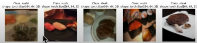
Turning custom-loaded images into DataLoader’s
from torch.utils.data import DataLoader
BATCH_SIZE = 32
NUM_WORKERS = os.cpu_count()
train_dataloader_custom = DataLoader(dataset=train_data_custom
                                     batch_size=BATCH_SIZE,
                                     num_workers=NUM_WORKERS,
                                     shuffle=True)
test_dataloader_custom = DataLoader(dataset=test_data_custom
                                     batch_size=BATCH_SIZE,
                                     num_workers=NUM_WORKERS,
                                     shuffle=False)
Other forms of transforms (data augmentation)
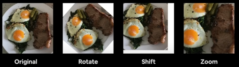
Data augmentation is the technique of intentionally increasing variation in your training data. In the case of picture data, this could include applying different image transformations to the training images.
from torchvision import transforms

train_trainsform = transforms.Compose([
  transforms.Resize(size=(224, 224)),
  transforms.TrivialAugmentWide(num_magnitude_bins=31),
  transforms.ToTensor()
])

test_transform = transforms.Compose([
  transforms.Resize(size=(224,224)),
  transforms.ToTensor()
])

image_path_list = list(image_path.glob("*/*/*.jpg"))

plot_transformed_images(
  image_paths = image_path_list,
  transform = train_transform,
  n = 3,
  seed = None
)
Random effects are applied to create data augmentation.
Model 0: TinyVGG without data augmentation
Let's recreate the TinyVGG architecture from the CNN Explainer website: poloclub.github.io/cnn-explainer
Creating transforms and loading data from Model 0
# Create simple transform
simple_transform = transforms.Compose([
                                        transforms.Resize(size=(64,64)),
                                        transform.ToTensor()
])

# Load and transform data
from torchvision import datasets
train_data_simple = datasets.ImageFolder(root=train_dir,
                                         transform=simple_transform)
test_data_simple = datasets.ImageFolder(root=test_dir,
                                        transform=simple_transform)

# Turn the dataset into DataLoaders
import os
from torch.utils.data import DataLoader

# Seting up batch size and number of works
BATCH_SIZE = 32
NUM_WORKERS = os.cpu_count()

# Create DataLoader's
train_dataloader_simple = DataLoader(dataset=train_data_simple,
                                      batch_size=BATCH_SIZE,
                                      shuffle=True,
                                      num_workers=NUM_WORKERS)
test_dataloader_simple = DataLoader(dataset=test_data_simple,
                                    batch_size=BATCH_SIZE,
                                    shuffle=False,
                                    num_workers=NUM_WORKERS)
class TinyVGG(nn.Module):
""" Model architecture copying TinyVGG from CNN Explainer."""
def __init__(self, input_shape: int, hidden_units:int, output_shape:int)->None:
super().__init__()
self.conv_block_1 = nn.Sequential(
nn.Conv2d(in_channels=hidden_units,
out_channels=hidden_units,
kernel_size=3,
stride=1,
padding=0)
nn.ReLU(),
nn.Conv2d(in_channels=hidden_units,
out_channels=hidden_units,
kernel_size=3,
stride=1,
padding=0)
nn.ReLU(),
nn.MaxPool2d(kernel_size=2,
stride=2) # default stride value is same as kernel_size
)
self.conv_block_2 = nn.Sequential(
nn.Conv2d(in_channels=hidden_units,
out_channels=hidden_units,
kernel_size=3,
stride=1,
padding=0)
nn.ReLU(),
nn.Conv2d(in_channels=hidden_units,
out_channels=hidden_units,
kernel_size=3,
stride=1,
padding=0)
nn.ReLU(),
nn.MaxPool2d(kernel_size=2,
stride=2) # default stride value is same as kernel_size
)
self.classifier = nn.Sequential(
nn.Flatten(),
nn.Linear(in_features=hidden_units*13*13,
out_features=output_shape)
)
def forward(self, x):
x = self.conv_block_1(x)
print(x.shape)
x = self.conv_block_2(x)
print(x.shape)
x = self.classifier(x)
print(x.shape)
return x
return self.classifier(self.conv_block_2(self.conv_block_1(x))) #benefits from operator fusiontorch.manual_seed(42)
model_0 = TinyVGG(input_shape=3,
hidden_units=10,
output_shape=len(class_Names)).to(device)Trying a forward pass on a single image (to the model)
# Get a single image batch
image_batch, label_batch = next(iter(train_dataloader_simple))
# Trying a forward pass
model_0(image_batch)
Use ‘torchinfo’ to get an idea of the shapes going through our model
try:
  import torchinfo
except:
  !pip install torchinfo
  import torchinfo

from torchinfo import summary
summary(model_0, input_size = [1, 3, 64, 64])
Creating train and test loop functions
train_step(): takes in a model and dataloader and trains the model on the dataloader.
test_step(): takes in a model and dataloader and evaluates the model on the dataloader.
# Create train_step()
def train_step(model: torch.nn.Module,
               data_loader: torch.utils.data.DataLoader,
               loss_fn: torch.nn.Module,
               optimizer: torch.optim.Optimizer,
               device=device):

model.train()

train_loss, train_acc = 0,0

for batch, (X,y) in enumerate(data_loader):
  X, y = X.to(device), y.to(device)

  y_pred = model(X)
  loss = loss_fn(y_pred, y)
  train_loss  += loss.item()

  optimizer.zero_grad()

  loss.backward()

  optimizer.step()


  y_pred_class = torch.argmax(torch.softmax(y_pred, dim=1), dim=1)

  train_acc += (y_pred_class==y).sum().item()/len(y_pred)


  train_loss = train_loss / len(data_loader)
  train_acc = train_acc / len(data_loader)

  return train_loss, train_acc


def test_step(model: torch.nn.Module,
               data_loader: torch.utils.data.DataLoader,
               loss_fn: torch.nn.Module,
               device=device):

model.eval()

test_loss, test_acc = 0,0

with torch.inference_mode():
  for batch, (X, y) in enumarate(data_loader):
    X, y = X.to(device), y.to(device)

    test_pred_logits = model(X)

    loss = loss_fn(test_pred_logits, y)
    test_loss += loss.item()

    test_pred_labels = test_pred_logits.argmax(dim=1)
    test_acc += ((test_pred_labels == y).sum().item()/len(test_pred_labels))

# Adjust metrics to get average loss and accuracy per batch
test_loss = test_loss / len(data_loader)
test_acc = test_acc / len(data_loader)
return test_loss, test_acc
Creating a train() function to combine train_step() and test_step()
from tqdm.auto import tqdm

# 1. Create a train funciton that takes in various
# model parameters + optimizer + dataloaders + loss function
def train(model: torch.nn.Module,
          train_dataloader: torch.utils.data.DataLoader,
          test_dataloader: torch.utils.data.DataLoader,
          optimizer: torch.optim.Optimizer,
          loss_fn: torch.nn.Module = nn.CrossEntropyLoss(),
          epochs: int = 5,
          device=device):

# 2. Create empty results dictionary
results = {"train_loss": [],
           "train_acc": [],
           "test_loss": [],
           "test_acc": []}

for epoch in tqdm(range(epochs)):
  train_loss, train_acc = train_step(model=model,
                                     data_loader=train_dataloader,
                                     loss_fn=loss_fn,
                                     optimizer=optimizer,
                                     device=device)

  test_loss, test_acc = test_step(model=model,
                                  data_loader=test_dataloader,
                                  loss_fn=loss_fn,
                                  device=device)


print(f"Epoch: {epoch} | Train loss: {train_loss:.4f}, Train acc: {train_acc:.4f}")

# 5. Update results dictionary
results["train_loss"].append(train_loss)
results["train_acc"].append(train_acc)
results["test_loss"].append(test_loss)
results["test_acc"].append(test_acc)


# 6. Return the filled results at the end of epochs
return results
Training and evaluating model 0
torch.manual_seed(42)
torch.cuda.manual_seed(42)

num_epochs = 5

model_5 = TinyVGG(input_shape=3, hidden_units=10, output_shape=len(train_data.classes)).to(device)

loss_fn = nn.CrossEntropyLoss()
optimizer = torch.optim.Adam(params=model_0.parameters(),
                             lr=0.001)

from timeit import default_timer as timer
start_time = timer()

model_0_results = train(model=model_0,
                        train_dataloader=train_dataloader_simple,
                        test_dataloader=test_dataloader_simple,
                        optimizer=optimizer,
                        loss_fn=loss_fn,
                        epochs=NUM_EPOCHS)


end_time = timer()
pritn(f"Total training time: {end_time-start_time:.3f} seconds")
Plotting the loss curves of Model 0
A loss curve is a method for tracking your model's progress over time.
model_0_results.keys() # dict_keys(['train_loss', 'train_acc', 'test_loss', 'test_acc']

def plot_loss_curves(rsults: Dict[str, List[float]]):
  """"Plots training curves of a results dictionary."""
  # Get the loss values of the results dicitionary(train and test)
  loss = results["train_loss"]
  test_loss = results["test_loss"]

  # Get the accuracy values of the results dictionary (training and test)
  accuracy = results["train_acc"]
  test_accuracy = results["test_acc"]

  # Figure out how many epochs there were
  epochs = range(len(results["train_loss"]))

  plt.figure(figsize=(15, 7))
  plt.subplot(1,2,1)
  plt.plot(epochs, loss, label="train_loss")
  plt.plot(epochs, loss, label="test_loss")
  plt.title("Loss")
  plt.title("Epochs")
  plt.legend()

  plt.subplot(1,2,2)
  plt.plot(epochs, accuracy, label="train_accuracy")
  plt.plot(epochs, test_accuracy, label="test_accuracy")
  plt.title("Accuracy")
  plt.xlabel("Epochs")
  plt.legend()

plot_loss_curves(model_0_results)
It's not so bad; the loss decreases over time but can be improved to look like an elbow.
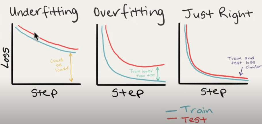
What should an ideal loss curve look like?
A loss curve is one of the most effective methods for troubleshooting a model.
The examples below demonstrate underfitting (not enough training), overfitting (too much training), and just right.
If your model is overfitting, what should you do?
- Get additional data: Gives a model a better chance to understand patterns between samples.
Data augmentation: Increase the variability of your training dataset without gathering more data (for example, randomly rotate your pizza photographs by 30 degrees). Increased diversity causes a model to learn more generalization patterns.
Find better data: Not all data samples are created equal. Removing bad samples or adding good ones to your dataset can help your model perform better.
Use Transfer Learning: Take a model's pre-learned patterns from one problem and modify them to fit your needs. For example, consider a model trained on images of vehicles to recognize photographs of trucks. - Simplify your model: If your present model is already overfitting the training data, it is likely that it is too sophisticated. This suggests it is learning the data's patterns too well and is unable to generalize to new data. One method for simplifying a model is to reduce the number of layers used or the number of hidden units in each layer.
Use learning rate decay. The goal here is to gradually decrease the learning rate as the model trains. This is similar to reaching for a coin in the back of a couch. As you draw closer, your steps become smaller. The same goes for the learning rate; the closer you come to convergence, the smaller your weight should be updates of your model. - If your model is underfitting, what should you do?
- Add more layers/units to your model: If your model is underfitting, it may not be able to learn the necessary patterns in the data to predict. One technique to improve the predictive power of your model is to increase the number of hidden layer units within those layers.
Tweak the learning rate: Perhaps your model's learning rate was set too high from the beginning. And it tries to update its weights too many times per epoch, resulting in little learning. In this situation, you may reduce the learning rate and see what occurs.
- Train for longer: A model may require more time to learn data representations. If you notice that your model isn't learning anything in your smaller experiments, leaving it to train for more epochs may result in improved performance.
Transfer learning: Take a model's pre-learned patterns from one problem and modify them to solve your own challenge. Consider using a model trained on vehicle images to recognize truck images.
Reduce regularization: Perhaps your model is underfitting because you're attempting to avoid overfitting too much. Holding back on regularization approaches can improve your model's fit to the data.
Model 1: TinyVGG with Data Augmentation
Let's try another modeling exercise, this time utilizing the same model but with some data augmentation.
Create transform with data augmentation
#Create training transform with TrivialAugment
from torchvision import transforms
train_transform_trivial = transforms.Compose([
                                               transforms.Resize(size=(64,64)),
                                               transforms.TrivialAugmentWide(numaginutude_bins=31),
                                               transforms.ToTensor()

])

test_transform_simple = transforms.Compose([
                                              transforms.Resize(size=(64,64)),
                                              transforms.ToTensor()
])
Create train and test Datasets and DataLoader’s with data augmentation
# Turn image folders into Datasets
from torchvision import datasets
train_data_augmented = datasets.ImageFolder(root=train_dir,
                                            transform=train_transform=trivial)
test_data_simple = datasets.ImageFolder(root=test_dir,
                                        transform=test_transform_simple)
# Turn our Datasets into DataLoaders
import os
from torch.utils.data import DataLoader
BATCH_SIZE = 32
NUM_WORKERS = os.cpu_count()
torch.manual_seed(42)
train_dataloader_augmented = DataLoader(dataset=train_data_augmented,
batch_size=BATCH_SIZE,
shuffle=True,
num_workers=NUM_WORKERS)
test_dataloader_augmented = DataLoader(dataset=test_data_augmented,
batch_size=BATCH_SIZE,
shuffle=True,
num_workers=NUM_WORKERS)Construct and train model 1
This time, we'll use the same model architecture, but with augmented training data.
# Create model_1 and send it to the target device
torch.manual_seed(42)
model_1 = TinyVGG(input_shape=3,
                  hidden_units=10,
                  output_shape=len(train_data_augmented.classes)).to(device)
Now we have a model and dataloaders let’s create a loss function and an optimizer and call upon our train() function to train and evaluate our model.
torch.manual_seed(42)
torch.cuda.manual_seed(42)

NUM_EPOCHS = 5

loss_fn = nn.CrossEntropyLoss()
optimizer = torch.optim.Adam(params=model_1.parameters(), lr=0.001)

from timeit import default_timer as timer
start_time = timer()

model_1_results = train(model=model_1,
                        train_Dataloader=train_dataloader_augmented,
                        test_dataloader=test_dataloader_simple,
                        optimizer=optimizer,
                        loss_fn=loss_fn,
                        epochs=NUM_EPOCHS,
                        device=device)

end_timer = timer()
print(f"Total training time for model_1: {end_time-start_time:.3f} seconds")
Plot the loss curves of model 1
A loss curve allows you to analyze your model's performance over time.
plot_loss_curves(model_1_results)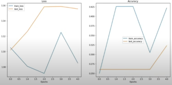
It did not get better.
Compare model results
After analyzing our modeling experiments independently, it is critical to compare them to one another.
There are a few different ways to do this:
- Hard coding (what we are doing)
- PyTorch + Tensorboard : pytorch.org/docs/stable/tensorboard.html
- Weights and Biases
- MLFlow
import pandas as pd
model_0_df = pd.DataFrame(model_0_results)
model_1_df = pd.DataFrame(model_1_results)

plt.figure(figsize=(15,10))
epochs = range(len(model_0_df))

plt.subplot(2,2,1)
plt.plot(epochs, model_0_df["train_loss"], loss="Model 0")
plt.plot(epochs, model_1_df["train_loss"], loss="Model 1")
plt.title("Train Loss")
plt.xlabel("Epochs")
plt.legend()

plt.subplot(2,2,2)
plt.plot(epochs, model_0_df["test_loss"], loss="Model 0")
plt.plot(epochs, model_1_df["test_loss"], loss="Model 1")
plt.title("Test Loss")
plt.xlabel("Epochs")
plt.legend()

plt.subplot(2,2,1)
plt.plot(epochs, model_0_df["train_acc"], loss="Model 0")
plt.plot(epochs, model_1_df["train_acc"], loss="Model 1")
plt.title("Train Acc")
plt.xlabel("Epochs")
plt.legend()

plt.subplot(2,2,2)
plt.plot(epochs, model_0_df["test_acc"], loss="Model 0")
plt.plot(epochs, model_1_df["test_acc"], loss="Model 1")
plt.title("Test Acc")
plt.xlabel("Epochs")
plt.legend()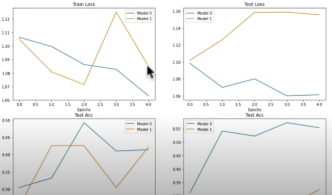
Making a prediction on a custom image
Although we trained a model using custom data, how can we forecast a sample image that is not part of the training or testing datasets?
import requests

custom_image_path = data_path / "04-pizza-dad.jpeg"

if not custom_image_path.is_file():
  with open(custom_image_path, "wb") as f:
    request = requests.get("https://raw.githubusercontent.com/mrdbourke/pytorch-deep-learning/main/images/05-pizza-dad.jpeg")
    print(f"Downloading {custom_image_path}...")
    f.write(request.content)
else:
  print(f"{custom_image_} already exists, skipping download...")
Loading in a custom image with PyTorch
We must ensure that our custom image matches the format of the data on which our model was trained.
- In tensor form with datatype(torch.float32)
- Of shape 64x64x3
- On the right device
import torchvision

custom_image_uint8 = torchvision.io.read_image(str(custom_image_path))
plt.imshow(custom_image_uint8.permute(1,2,0))
Making a prediction on a custom image with a trained Pytorch model
Let's make a forecast on an image in uint8 format.
from torchvision import transforms
custom_image_transform = transforms.Compose([transforms.Resize(size=(64,64))])

custom_image_transformed = custom_image_transform(custom_image)
plt.imshow(custom_image_transformed.permute(1,2,0))


model_1.eval()
with torch.inference_mode():
  custom_image_pred = model_1(custom_image_transformed.unsqueeze(0).to(device))
custom_image_pred
Note: To predict a bespoke image, we have to:
- Load the image and turn it into a tensor
- Make sure the image is the same datatype as the model(torch.float32)
- Make sure the image is the same shape as the data the model was trained on (3,64,64) with a batch size (1,3,64,64)
- Make sure the image is on the same device as our model
# Convert logits to prediction probabilities
custom_image_pred_probs = torch.softmax(custom_image_pred, dim=1)
custom_image_pred_labels = torch.argmax(custom_image_pred_probs, dim=1)
Putting custom image prediction together: building a function
The ideal outcome is a function that accepts an image path, has our model predict that image, and plots the image and prediction.
def pred_and_plot_image(model:torch.nn.Module,
                        image_path:str,
                        class_Names: List[str] = None,
                        transform=None,
                        device=device):
# Load in the image
target_image = torchvision.io.read_image(str(image_path)).type(torch.float32)
#Divide the image pixel values by 255 to get them between 0 and 1
target_image = target_image / 255
# Transform if necessary
if transform:
  target_image = transform(target_image)
# Make sure the model is on the target device
model.to(device)

# Turn on eval/inference mode and make a prediction
model.eval()
with torch.inference_mode():
  # Add an extra dimension to the image (this is the batch dimension e.g our model will predict on batches of lx image)
  target_image = target_image.unsqueeze(0)
  # Make a prediction on the iamge with an extra dimension
  target_image_pred = model(target_image_pred.to(device))

# Covnert logits -> prediction probabilities
target_image_pred_probs = torch.softmax(target_image_pred, dim=1)

# Convert prediction probabilities -> prediciton labels
target_image_pred_labels = torch.argmax(target_image_pred_probs, dim=1)

# Plot the image alongside the prediciton and prediction probability
plt.imshow(target_image.squeeze().permute(1,2,0)) # Remove batch dimension and rearange shape
if class_names:
  title = f"Pred: {class_names[target_image.cpu()]} | Prob: {target_image_pred_probs.max().cpu():.3f}"
else:
  title = f"Pred: {target_image_pred_label} | Prob: {target_image_pred_probs.max().cpu():.3f}"
plt.title(title)
plt.axis(False)pred_and_plot_image(model=model_1,
image_path=custom_image_path,
class_names=class_names,
transform=custom_image_transform,
device=device)
We have reached the conclusion of this series. Now you understand what Pytorch is and how it works. You also have application examples in the visual usage sections.
What's next?
- Transfer learning
- Model deployment
- Paper replicating
- Going modular
- Experiment tracking
Resource
[1] freeCodeCamp.org, (6 Ekim 2022), PyTorch for Deep Learning & Machine Learning — Full Course:


0 Comments