
Embedding models generate embedding vectors, which enable the development of semantic or meaning-based retrieval systems. This article will discuss the history of embedding models, as well as the detailed technical design and implementation. This is a technical article that discusses the building components rather than the applications. You may have heard that Embedding Vectors are employed in Generative AI applications. These vectors are fantastic for capturing the sense of a word or phrase. The founders of Vectara will explain how these embedding models function. Vectara creates embedding models for use in RAG and other applications.
Training an embedding model is tricky since you want to use a large amount of existing text as training data. Initially, the idea of using surrounding words as clues was discussed. This methodology was popularized by Mikolov, Chen, Corrado, and Dean's embedding model word2vec, which was then enhanced by Pennington, Socha, and Manning at Stanford University's GloVe method.
Previously, RNNs such as LSTM were used to produce more accurate embeddings by extending the context window surrounding the word. Transformers were introduced in 2017 to enable the usage of feedforward neural networks, which allow RNNs to efficiently process sequential data. The BERT model, which was launched the following year, is a deep transformer network trained to fill in missing words in order to obtain deep language understanding, and it marked the beginning of the contemporary era of NLP. You can also analyze more than one word or sentence.
You may also refine these embedding models to evaluate sentences. Let's first learn about embedding models and how they're utilized, followed by BERT (a two-way transformer). BERT is utilized in a variety of applications, but we will focus on retrieval. We will learn how to design and apply a contrastive loss to train a dual-encoder model suitable for RAG applications. One encoder is trained for inquiries, and another for responses.
Introduction to Embedding Models
Vector embeddings transform real-world items, such as a neighbourhood, a sentence, or an image, into vector representations or points in a vector space. This representation is distinguished by the fact that points in the vector space that are comparable in some sense have similar semantic meanings.
Word2vec is a ground-breaking study in learning token or word embeddings that preserve semantic meaning, demonstrating that dense vector-based representations of words can capture their semantic meanings. What's remarkable is that these word embeddings behave like vectors in a vector space, allowing you to apply algebraic equations and operations to them.
The equation "queen — woman + man = king" has "king" as the closest vector. Training on the Star Wars text can result in phrases like "Yoda—good + evil = Vader".
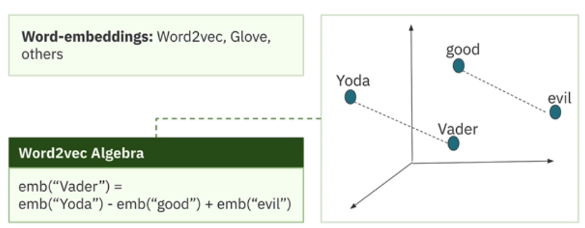
A sentence embedding model uses the same idea to represent full sentences. It converts a sentence into a numerical vector that represents the complete sentence's semantic content.

This tutorial focuses on text embeddings. However, embeddings are a broad idea that can be applied and employed in a variety of fields. For example, deep learning models can be trained to learn embeddings for photos, movies, and audio samples.
Image embeddings convert visual content into a vector format.
Video embeddings preserve the features of video data, such as visual appearance and temporal dynamics.
Audio embeddings encode audio signals in a vector space.
Graph embeddings convert nodes, edges, and their characteristics into a vector space while keeping structural information.
One of the most widely used multimodal embeddings is OpenAI's CLIP model, which aligns images and text in a shared representation space and can perform a number of tasks. For example, generate words from photos. Let's look at a few uses of vector embeddings.
Token embeddings are used to represent tokens in transformer models while creating Large Language Models (LLMs).
Sentence embeddings allow for efficient retrieval of relevant sections in RAG applications.
Its utility for recommender systems arises from its ability to represent items in the embedding space and do similarity searches.
Anomaly detection finds data patterns that differ significantly from the norm.
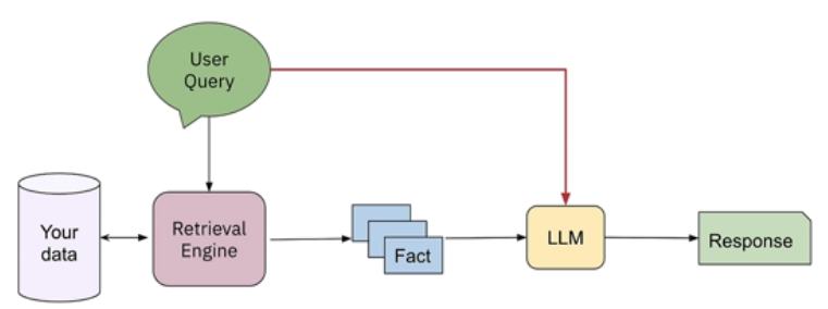
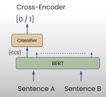
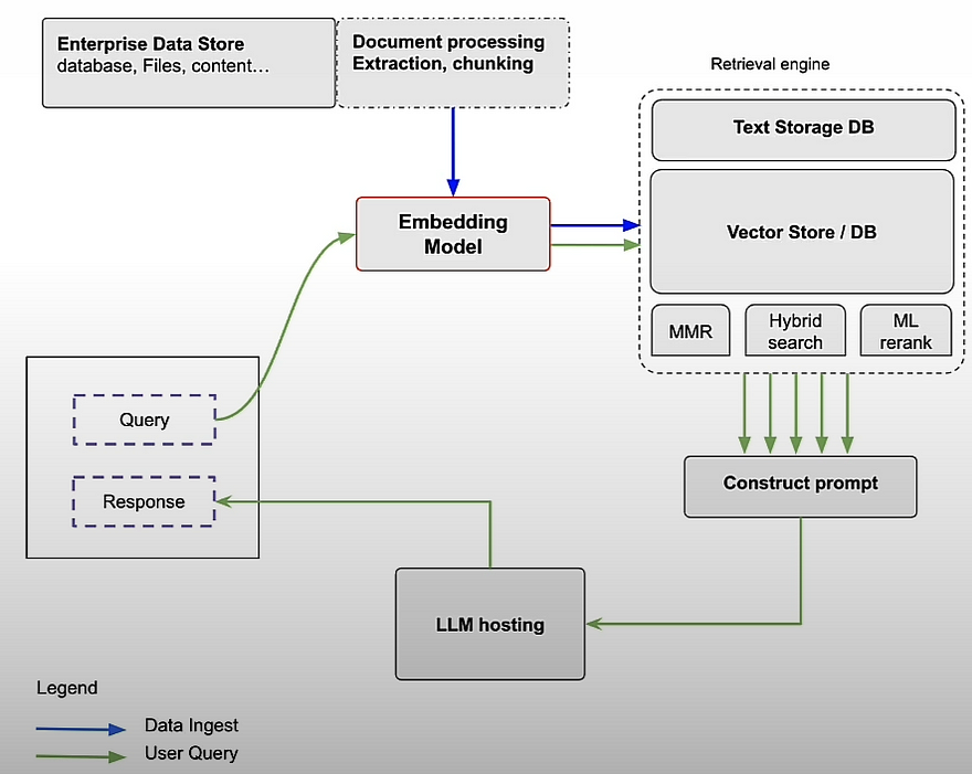
The retrieval engine is an important component of any well-designed RAG pipeline. Given a user question, you rank all available factors or text chunks based on their relevancy to the query before submitting the information to the LLM for a response. You might be wondering what algorithm we can apply for best retrieval. A cross-encoder is one method for rating text chunks based on their relevance. A cross-encoder is a transformer-based neural network model that functions as a classifier to identify relevance. Cross encoders are accurate, but slow. You use an encoder like BERT to concatenate the question and response with a separator token, then ask the cross-encoder to calculate the relevance of the answer to the query.

Cross encoders are extremely slow, and this method requires you to perform this classification step for each text chunk in your dataset. So this is not scalable. Sentence embedding models offer an option. This works as follows.
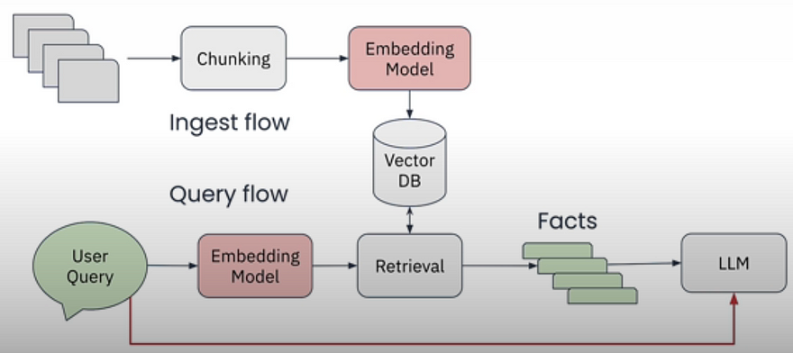
During indexing, you generate an embedding for each text segment and store it in a vector database. When a user submits a query, you use similarity search to find the most relevant chunks to retrieve. This is frequently less accurate than cross encoders, but it is significantly faster and offers a feasible and practical implementation approach.
Contextualized Token Embeddings
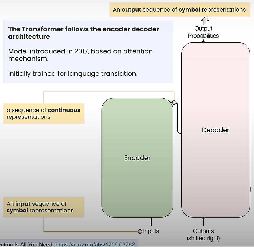
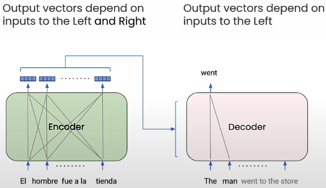
The following describes how a translation task would function. The encoder would accept phrases in one language and generate output vectors representing the meaning of the input phrase. To generate these vectors, the encoder could target tokens to the left or right of any given token. In contrast, the decoder operates a token at a time and considers the predicted tokens so far along with the outputs of the encoder.
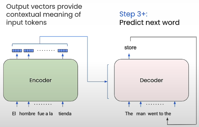
The encoder focuses on the tokens to the left and right of the output it generates. This leads to encoder output vectors that are contextualized vectors. In contrast, the decoder just looks at the inputs on the left. However, transformers with attention were utilized for more than only translation. Most popular LLMs, such as ChatGPT, use a decoder-only design. And BERT is an encoder-only transformer model that is commonly utilized as a component in phrase embedding models.
BERT was designed in two sizes: BERT Base had 12 layers, 768 hidden units, 12 attention heads, and 110 million parameters, while BERT Large had 24 layers, 1024 hidden units, 16 attention heads, and 340 million parameters. BERT was pre-trained on 3.3 billion words and is frequently utilized with extra task-specific fine-tuning steps.
The BERT was pre-trained for two tasks. The first duty is called Masked Language Modelling, or MLM. The inputs are phrases that begin with a special token called CLS and end with a separator token, SEP.
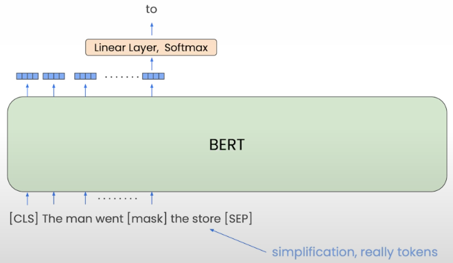
15% of all Wordpiece tokens are randomly disguised. The model must predict the disguised token. The model can employ both the Left and Right contexts. The task teaches the model to create contextualized word embeddings.
The second challenge is Next Sentence Prediction (NSP). The model guesses which sentences are likely to follow the supplied sentence.
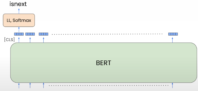
After that, you may apply the concept of transfer learning to BERT and fine-tune it for specific tasks like categorization, named entity identification, or question answering.
The cross encoder is a classifier that accepts two phrases separated by a special SEP token. The classifier was then asked to calculate the semantic similarity between the two sentences.
import warnings
warnings.filterwarnings('ignore')

import numpy as np
import matplotlib.pyplot as plt
from sklearn.decomposition import PCA
import torch

from transformers import BertTokenizer, BertModel
from sklearn.metrics.pairwise import cosine_similarity

# GloVe word embeddings
import gensim.downloader as api
word_vectors = api.load('glove-wiki-gigaword-100')
#word_vectors = api.load('word2vec-google-news-300')
word_vectors['king'].shape # (100,)
word_vectors['king'][:20]
# Words to visualize
words = ["king", "princess", "monarch", "throne", "crown",
         "mountain", "ocean", "tv", "rainbow", "cloud", "queen"]

# Get word vectors
vectors = np.array([word_vectors[word] for word in words])
# Reduce dimensions using PCA
pca = PCA(n_components=2)
vectors_pca = pca.fit_transform(vectors)
# Plotting
fig, axes = plt.subplots(1, 1, figsize=(5, 5))
axes.scatter(vectors_pca[:, 0], vectors_pca[:, 1])
for i, word in enumerate(words):
    axes.annotate(word, (vectors_pca[i, 0]+.02, vectors_pca[i, 1]+.02))
axes.set_title('PCA of Word Embeddings')
plt.show()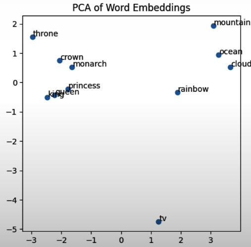
# Word2Vec algebra
result = word_vectors.most_similar(positive=['king', 'woman'],
                                   negative=['man'], topn=1)

# Output the result
print(f"""
    The word closest to 'king' - 'man' + 'woman' is: '{result[0][0]}'
    with a similarity score of {result[0][1]}""") # 0.769854

# GloVe vs BERT: Words in context
tokenizer = BertTokenizer.from_pretrained('./models/bert-base-uncased')
model = BertModel.from_pretrained('./models/bert-base-uncased')

# Function to get BERT embeddings
def get_bert_embeddings(sentence, word):
    inputs = tokenizer(sentence, return_tensors='pt')
    outputs = model(**inputs)
    last_hidden_states = outputs.last_hidden_state
    word_tokens = tokenizer.tokenize(sentence)
    word_index = word_tokens.index(word)
    word_embedding = last_hidden_states[0, word_index + 1, :]  # +1 to account for [CLS] token
    return word_embedding

sentence1 = "The bat flew out of the cave at night."
sentence2 = "He swung the bat and hit a home run."

word = "bat"

bert_embedding1 = get_bert_embeddings(sentence1, word).detach().numpy()
bert_embedding2 = get_bert_embeddings(sentence2, word).detach().numpy()
word_embedding = word_vectors[word]
print("BERT Embedding for 'bat' in sentence 1:", bert_embedding1[:5])
print("BERT Embedding for 'bat' in sentence 2:", bert_embedding2[:5])
print("GloVe Embedding for 'bat':", word_embedding[:5])

bert_similarity = cosine_similarity([bert_embedding1], [bert_embedding2])[0][0]
word_embedding_similarity = cosine_similarity([word_embedding], [word_embedding])[0][0]

print(f"Cosine Similarity between BERT embeddings in different contexts: {bert_similarity}")
print(f"Cosine Similarity between GloVe embeddings: {word_embedding_similarity}")
# Cross Encoder
from sentence_transformers import CrossEncoder
model = CrossEncoder('cross-encoder/ms-marco-MiniLM-L-6-v2', max_length=512,
                     default_activation_function=torch.nn.Sigmoid())
question = "Where is the capital of France?"
# Define sentences to compare
answers = [
    "Paris is the capital of France.",
    "Berlin is the capital of Germany.",
    "Madrid is the capital of Spain."
]
scores = model.predict([(question, answers[0]), (question, answers[1]),
                        (question, answers[2])])
print(scores)
most_relevant_idx = torch.argmax(torch.tensor(scores)).item()
print(f"The most relevant passage is: {answers[most_relevant_idx]}")
# [0.99965715 0.05289614 0.04520676]
# The most relevant passage is: Paris is the capital of France.
Token vs. Sentence Embedding
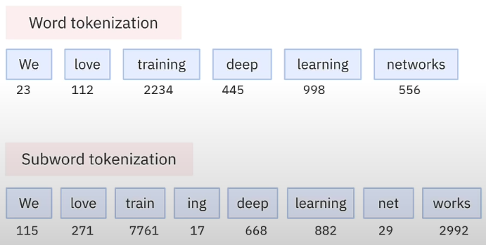
NLP systems work using tokens, which can be a word, a subword, or any sequence of characters. Subword tokenization strategies include BPE (Byte Pair Encoding), word piece, and sentence piece.
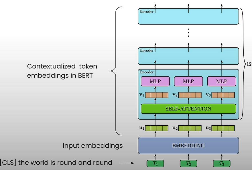
Let us investigate how token embeddings operate in BERT, which has a vocabulary of approximately 30k tokens and an embedding dimension of 768. The tokenizer input phrase is prefixed with a unique initial token named CLS, and all tokens are turned to token embeddings. Think of the first level of embeddings as fixed token embeddings that simply focus on the word itself. Each encoder layer in BERT produces embeddings for each token in the input sequence, but these embeddings now include information about the rest of the phrase, which we refer to as contextualized embeddings. As we progress through the layers, these representations improve their ability to integrate context from the entire phrase.
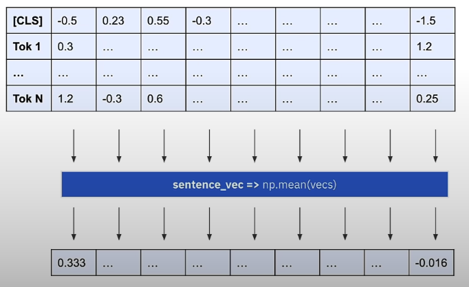
After receiving word embeddings such as GloVe or Word2Vec, researchers attempted to obtain sentence embeddings such as cosine similarity or dot product similarity. Initial methods were rudimentary; some attempted to average the output embeddings of the final layer of a transformer model of all tokens in the sentence, commonly known as mean pooling. Others attempted to represent the statement simply by embedding the CLS token. Each of these attempts failed.
# SETUP

# Warning control
import warnings
warnings.filterwarnings('ignore')
import torch
import numpy as np
import seaborn as sns
import pandas as pd
import scipy
from transformers import BertModel, BertTokenizer
from datasets import load_dataset

model_name = "./models/bert-base-uncased"
tokenizer = BertTokenizer.from_pretrained(model_name)
model = BertModel.from_pretrained(model_name)

# Mean pooling. Encodes sentence to tokens, creates attention mask, runs through BERT, gets output
# and mean pools to get to the final  output.
def get_sentence_embedding(sentence):
    encoded_input = tokenizer(sentence, padding=True, truncation=True, return_tensors='pt')
    attention_mask = encoded_input['attention_mask']   # to indicate which tokens are valid and which are padding

    # Get the model output (without the specific classification head)
    with torch.no_grad():
        output = model(**encoded_input)

    token_embeddings = output.last_hidden_state
    input_mask_expanded = attention_mask.unsqueeze(-1).expand(token_embeddings.size()).float()

    # mean pooling operation, considering the BERT input_mask and padding
    sentence_embedding = torch.sum(token_embeddings * input_mask_expanded, 1) / torch.clamp(input_mask_expanded.sum(1), min=1e-9)

    return sentence_embedding.flatten().tolist()

# Normalize each row and creates cosine similarity
def cosine_similarity_matrix(features):
    norms = np.linalg.norm(features, axis=1, keepdims=True)
    normalized_features = features / norms
    similarity_matrix = np.inner(normalized_features, normalized_features)
    rounded_similarity_matrix = np.round(similarity_matrix, 4)
    return rounded_similarity_matrix

# plot similarity matrix with heatmap
def plot_similarity(labels, features, rotation):
    sim = cosine_similarity_matrix(features)
    sns.set_theme(font_scale=1.2)
    g = sns.heatmap(sim, xticklabels=labels, yticklabels=labels, vmin=0, vmax=1, cmap="YlOrRd")
    g.set_xticklabels(labels, rotation=rotation)
    g.set_title("Semantic Textual Similarity")
    return g

# TOKEN EMBEDDINGS
messages = [
    # Smartphones
    "I like my phone",
    "My phone is not good.",
    "Your cellphone looks great.",

    # Weather
    "Will it snow tomorrow?",
    "Recently a lot of hurricanes have hit the US",
    "Global warming is real",

    # Food and health
    "An apple a day, keeps the doctors away",
    "Eating strawberries is healthy",
    "Is paleo better than keto?",

    # Asking about age
    "How old are you?",
    "what is your age?",
]
embeddings = []
for t in messages:
    emb = get_sentence_embedding(t)
    embeddings.append(emb)

plot_similarity(messages, embeddings, 90)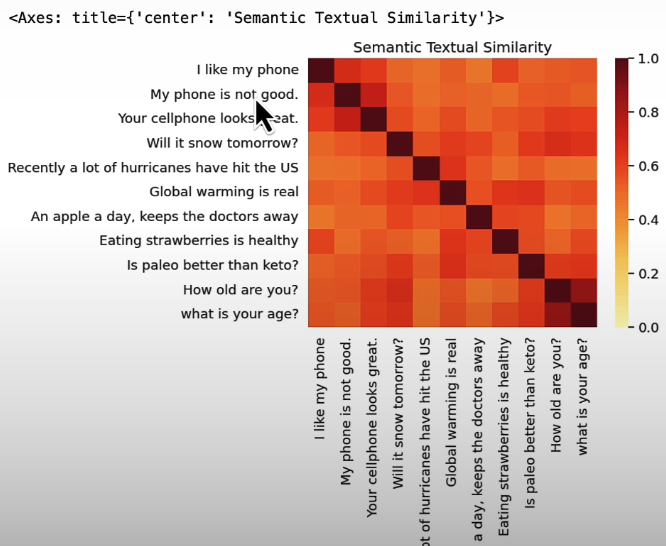
sts_dataset = load_dataset("mteb/stsbenchmark-sts")
sts = pd.DataFrame({'sent1': sts_dataset['test']['sentence1'],
                    'sent2': sts_dataset['test']['sentence2'],
                    'score': [x/5 for x in sts_dataset['test']['score']]})
sts.head(10) # Grand truth and similarity score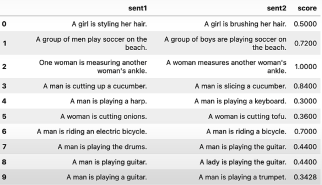
"""
About the scores: These scores are based on human evaluations and in the range 0 to 5 (see https://aclanthology.org/S17-2001.pdf table 1 for how they work). For example "A woman is cutting onions" vs "A woman is cutting tofu" can be considered by a human as in between 2-3 or so. The goal of STS is more to show another example where instead of just our intuition there is some kind of human labeled dataset, albeit it's not exactly a similarity in the sense of cosine but according to the rules of table 1 in the paper above.
"""
def sim_two_sentences(s1, s2):
    emb1 = get_sentence_embedding(s1)
    emb2 = get_sentence_embedding(s2)
    sim = cosine_similarity_matrix(np.vstack([emb1, emb2]))
    return sim[0,1]

n_examples = 50

sts = sts.head(n_examples)
sts['avg_bert_score'] = np.vectorize(sim_two_sentences) \
                                    (sts['sent1'], sts['sent2'])
sts.head(10)
pc = scipy.stats.pearsonr(sts['score'], sts['avg_bert_score'])
print(f'Pearson correlation coefficient = {pc[0]}\np-value = {pc[1]}')
# Pearson correlation coefficient= 0.3210017220269546
# p-value = 0.02103013509739929
# We are sure mean pooling's no variation works.

# BETTER APPROACH: SBERT AND DUAL ENCODERS
from sentence_transformers import SentenceTransformer
model = SentenceTransformer("sentence-transformers/all-MiniLM-L6-v2")
embeddings = []
for t in messages:
    emb = list(model.encode(t))
    embeddings.append(emb)

plot_similarity(messages, embeddings, 90)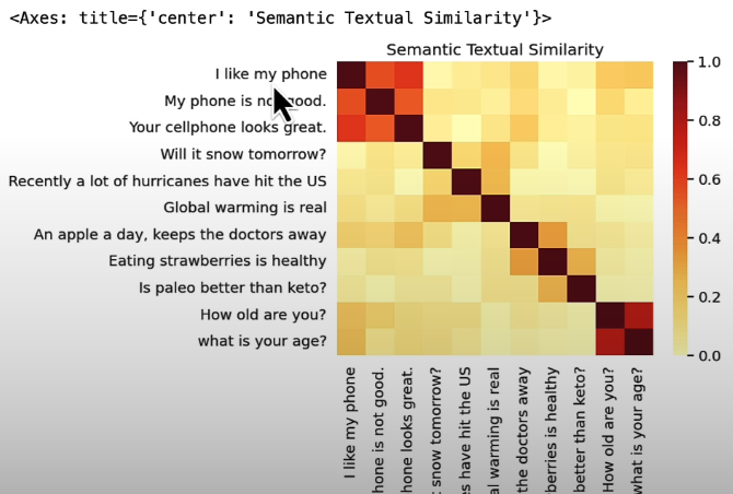
def sim_two_sentences(s1, s2):
    emb1 = list(model.encode(s1))
    emb2 = list(model.encode(s2))
    sim = cosine_similarity_matrix(np.vstack([emb1, emb2]))
    return sim[0,1]

sts['mini_LM_score'] = np.vectorize(sim_two_sentences)(sts['sent1'], sts['sent2'])
sts.head(10)
pc = scipy.stats.pearsonr(sts['score'], sts['mini_LM_score'])
print(f'Pearson correlation coefficient = {pc[0]}\np-value = {pc[1]}')
# Pearson correlation coefficient= 0.930374067376042
# p-value = 1.4823857251916192e-22
# This approach for sentence embeddings really working
Real progress in sentence embedding research began in 2018 when Google introduced Universal Sentence Encoder, which was built on the original transformer architecture. SBERT was the first model to be trained using data containing sentence pairs. The work on SBERT (Rimers and Gurevych) in 2019 quickly led to more innovation in the following years, with additional designs such as DPR (Dense Passage Retrieval), by Facebook and Sentence T5 (T5 model variant specifically trained for sentence embedding), E5, DRAGON in 2023 (technique that uses large scale synthetic data and curriculum learning to improve retrieval performance with sentence embedding models), COLBERT (multiple vectors to represent sentence embeddings an
While building sentence encoders, there are two conceivable goals. The first is pure sentence similarity, which involves employing embeddings to discover comparable items. The second step is to rank relevant sentences in response to a question, such as in RAG. They do not share the same goal. Take a look at the sample below to understand the difference. In RAG, the document should contain the potential answer to the inquiry rather than the query itself.
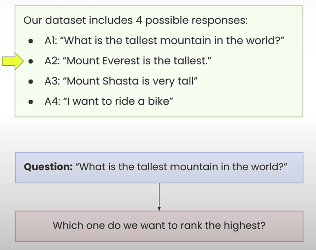
This results in a dual or bi-encoder architecture, which has two distinct encoders: the question encoder and the response encoder. The model is trained using contrastive loss.
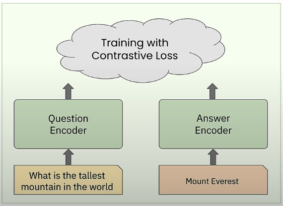
Training a Dual Encoder
We'll learn how to create a dual encoder in PyTorch and train it on a dataset of question-and-answer pairs. Let's look at the dual encoder architecture used to train sentence embedding models. During training, we use the CLS embedding vector from the final layer of each BERT encoder model to represent the question or answer, respectively. The dot product similarity between them shows a semantic match. A high number indicates that the answer is semantically related to the query, whereas a low value implies that it is not.
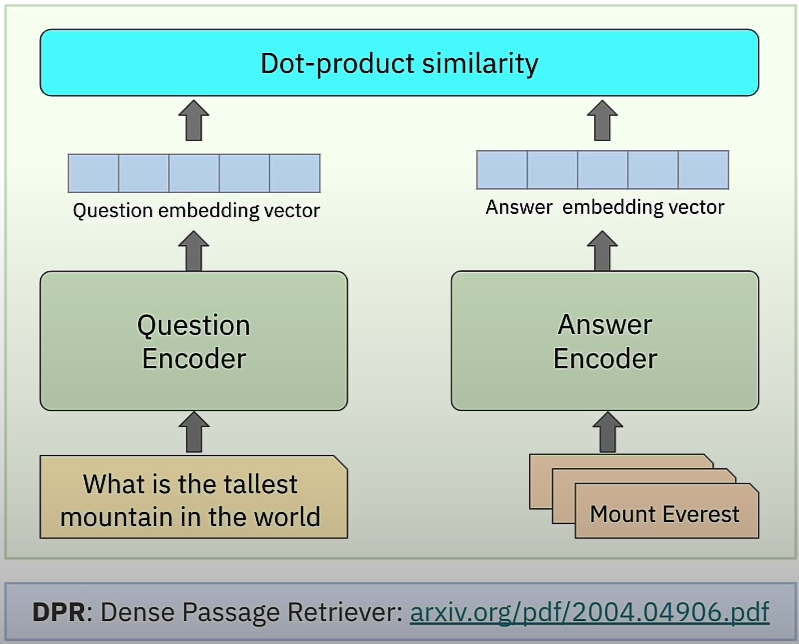
The dual encoder architecture employs contrastive loss. Contrastive loss is designed to ensure that embeddings of similar or positive pairs of data points are closer together in the embedding space than representations of dissimilar or negative pairs. The loss function promotes the model to maximize the similarity between embeddings of positive pairings while minimizing the similarity between negative ones.

- y(i,j) = 1 When question i and answer j are a match.
- sim(UI, vj) Similarity between embeddings of question i and answer j
- m margin parameter that defines the minimum acceptable distance between dissimilar pairs.
In our situation, a positive pair consists of the embeddings of a question and its correct response, whereas a negative pair consists of a question and any other incorrect answer in the batch.
The following is an example of contrastive loss:
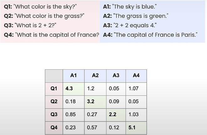
We obtained a single loss based on this 4x4 matrix, which decreases when the softmax values on the diagonal approach one and the remainder near zero.

In PyTorch, we employ a tiny trick with the cross entropy loss function to achieve one specific type of contrastive loss that works well in practice. N is the batch size, and loss_fn equals torch.nn.CrossEntropyLoss(); target = torch.arange(N); loss = loss_fn(similarity_scores,target). In code, we set the target argument of the cross entropy loss function to zero, one, two, and so on until n minus one, where n is the batch size.
This informs the cross entropy loss that the correct class, in this case the answer for each row, which is the query, is the one connected with it; in other words, A1 is the correct class for Q1, A2 is for Q2, and so on. In this method, we apply cross-entropy loss to get the desired contrastive loss. The employment of the softmax in the loss function promotes the exponent Sii. The similarity between inquiry i and answer I is great, implying that right pairs are also comparable. An exponent of Sij, where i and j are not the same, is small, which is exactly what we want with contrastive learning.
# Warning control
import warnings
warnings.filterwarnings('ignore')
import torch
import numpy as np
import pandas as pd
from transformers import AutoTokenizer

# The CrossEntropyLoss trick
df = pd.DataFrame(
    [
        [4.3, 1.2, 0.05, 1.07],
        [0.18, 3.2, 0.09, 0.05],
        [0.85, 0.27, 2.2, 1.03],
        [0.23, 0.57, 0.12, 5.1]
    ]
)
data = torch.tensor(df.values, dtype=torch.float32)

def contrastive_loss(data):
    target = torch.arange(data.size(0))
    loss = torch.nn.CrossEntropyLoss()(data, target)
    return loss

torch.nn.Softmax(dim=1)(data)
torch.nn.Softmax(dim=1)(data).sum(dim=1)
N = data.size(0)
non_diag_mask = ~torch.eye(N, N, dtype=bool)

for inx in range(3):
    data = torch.tensor(df.values, dtype=torch.float32)
    data[range(N), range(N)] += inx*0.5
    data[non_diag_mask] -= inx*0.02
    print(data)
    print(f"Loss = {contrastive_loss(data)}")

# The encoder module
class Encoder(torch.nn.Module):
    def __init__(self, vocab_size, embed_dim, output_embed_dim):
        super().__init__()
        self.embedding_layer = torch.nn.Embedding(vocab_size, embed_dim)
        self.encoder = torch.nn.TransformerEncoder(
            torch.nn.TransformerEncoderLayer(embed_dim, nhead=8, batch_first=True),
            num_layers=3,
            norm=torch.nn.LayerNorm([embed_dim]),
            enable_nested_tensor=False
        )
        self.projection = torch.nn.Linear(embed_dim, output_embed_dim)

    def forward(self, tokenizer_output):
        x = self.embedding_layer(tokenizer_output['input_ids'])
        x = self.encoder(x, src_key_padding_mask=tokenizer_output['attention_mask'].logical_not())
        cls_embed = x[:,0,:]
        return self.projection(cls_embed)
def train_loop(dataset):
    embed_size = 512
    output_embed_size = 128
    max_seq_len = 64
    batch_size = 32

    # define the question/answer encoders
    tokenizer = AutoTokenizer.from_pretrained('bert-base-uncased')
    question_encoder = Encoder(tokenizer.vocab_size, embed_size,
                               output_embed_size)
    answer_encoder = Encoder(tokenizer.vocab_size, embed_size,
                             output_embed_size)

    dataloader = torch.utils.data.DataLoader(dataset, batch_size=batch_size,
                                             shuffle=True)
    optimizer = torch.optim.Adam(
        list(question_encoder.parameters()) + list(answer_encoder.parameters()
    ), lr=1e-5)
    loss_fn = torch.nn.CrossEntropyLoss()

    running_loss = []
    for _, data_batch in enumerate(dataloader):

        # Tokenize the question/answer pairs (each is a batch of 32 questions and 32 answers)
        question, answer = data_batch
        question_tok = tokenizer(question, padding=True, truncation=True, return_tensors='pt', max_length=max_seq_len)
        answer_tok = tokenizer(answer, padding=True, truncation=True, return_tensors='pt', max_length=max_seq_len)

        # Compute the embeddings: the output is of dim = 32 x 128
        question_embed = question_encoder(question_tok)
        answer_embed = answer_encoder(answer_tok)

        # Compute similarity scores: a 32x32 matrix
        # row[N] reflects similarity between question[N] and answers[0...31]
        similarity_scores = question_embed @ answer_embed.T

        # we want to maximize the values in the diagonal
        target = torch.arange(question_embed.shape[0], dtype=torch.long)
        loss = loss_fn(similarity_scores, target)
        running_loss += [loss.item()]

        # this is where the magic happens
        optimizer.zero_grad()    # reset optimizer so gradients are all-zero
        loss.backward()
        optimizer.step()

    return question_encoder, answer_encoder

# Training in multiple Epochs
def train(dataset, num_epochs=10):
    embed_size = 512
    output_embed_size = 128
    max_seq_len = 64
    batch_size = 32

    n_iters = len(dataset) // batch_size + 1

    # define the question/answer encoders
    tokenizer = AutoTokenizer.from_pretrained('bert-base-uncased')
    question_encoder = Encoder(tokenizer.vocab_size, embed_size, output_embed_size)
    answer_encoder = Encoder(tokenizer.vocab_size, embed_size, output_embed_size)

    # define the dataloader, optimizer and loss function
    dataloader = torch.utils.data.DataLoader(dataset, batch_size=batch_size, shuffle=True)
    optimizer = torch.optim.Adam(list(question_encoder.parameters()) + list(answer_encoder.parameters()), lr=1e-5)
    loss_fn = torch.nn.CrossEntropyLoss()

    for epoch in range(num_epochs):
        running_loss = []
        for idx, data_batch in enumerate(dataloader):

            # Tokenize the question/answer pairs (each is a batc of 32 questions and 32 answers)
            question, answer = data_batch
            question_tok = tokenizer(question, padding=True, truncation=True, return_tensors='pt', max_length=max_seq_len)
            answer_tok = tokenizer(answer, padding=True, truncation=True, return_tensors='pt', max_length=max_seq_len)
            if inx == 0 and epoch == 0:
                print(question_tok['input_ids'].shape, answer_tok['input_ids'].shape)

            # Compute the embeddings: the output is of dim = 32 x 128
            question_embed = question_encoder(question_tok)
            answer_embed = answer_encoder(answer_tok)
            if inx == 0 and epoch == 0:
                print(question_embed.shape, answer_embed.shape)

            # Compute similarity scores: a 32x32 matrix
            # row[N] reflects similarity between question[N] and answers[0...31]
            similarity_scores = question_embed @ answer_embed.T
            if inx == 0 and epoch == 0:
                print(similarity_scores.shape)

            # we want to maximize the values in the diagonal
            target = torch.arange(question_embed.shape[0], dtype=torch.long)
            loss = loss_fn(similarity_scores, target)
            running_loss += [loss.item()]
            if idx == n_iters-1:
                print(f"Epoch {epoch}, loss = ", np.mean(running_loss))

            # this is where the magic happens
            optimizer.zero_grad()    # reset optimizer so gradients are all-zero
            loss.backward()
            optimizer.step()

    return question_encoder, answer_encoder

# Let's train
class MyDataset(torch.utils.data.Dataset):
    def __init__(self, datapath):
        self.data = pd.read_csv(datapath, sep="\t", nrows=300)

    def __len__(self):
        return len(self.data)

    def __getitem__(self, idx):
        return self.data.iloc[idx]['questions'], self.data.iloc[idx]['answers']

dataset = MyDataset('./shared_data/nq_sample.tsv')
dataset.data.head(5)

qe, ae = train(dataset, num_epochs=10)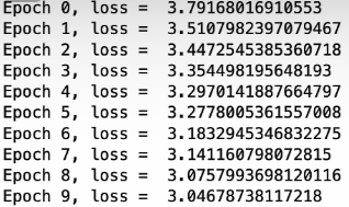
question = 'What is the tallest mountain in the world?'
tokenizer = AutoTokenizer.from_pretrained('bert-base-uncased')
question_tok = tokenizer(question, padding=True, truncation=True, return_tensors='pt', max_length=64)
question_emb = qe(question_tok)[0]
print(question_tok)
print(question_emb[:5])
answers = [
    "What is the tallest mountain in the world?",
    "The tallest mountain in the world is Mount Everest.",
    "Who is donald duck?"
]
answer_tok = []
answer_emb = []
for answer in answers:
    tok = tokenizer(answer, padding=True, truncation=True, return_tensors='pt', max_length=64)
    answer_tok.append(tok['input_ids'])
    emb = ae(tok)[0]
    answer_emb.append(emb)

print(answer_tok)
print(answer_emb[0][:5])
print(answer_emb[1][:5])
print(answer_emb[2][:5])
question_emb @ torch.stack(answer_emb).T
Using Embeddings in RAG
We'll learn how to use encoders in production, as well as how question and answer encoders work in a retrieval pipeline like the RAG system. We trained a dual encoder in the previous chapter, and now we have a question and answer encoder. As seen on the next page, during intake, we encode each text chunk using the response encoder and save the resulting vector embedding to the vector database.

When a user submits a query, we use the question encoder to create the query embedding vector. That vector is then utilized to retrieve the relevant facts or text segments, which are delivered to the LLM as part of the RAG flow.
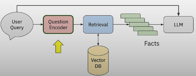
Neural/Vector search: Unable to compute similarity against all chunks: sim(q, a(i)), i=1,..., 1M. ANN (Approximate Nearest Neighbor) to the rescue! HNSW, Annoy, FAISS, and NMSLib are all algorithms and systems that use ANN. In production, you must add persistence when switching these algorithms from in-memory to on-disk vector storage.
# Warning control
import warnings
warnings.filterwarnings('ignore')
import numpy as np
from sentence_transformers import SentenceTransformer
from transformers import AutoTokenizer, DPRContextEncoder, DPRQuestionEncoder # DPR packages are for dual encoders
import logging

logging.getLogger("transformers.modeling_utils").setLevel(logging.ERROR)

def cosine_similarity_matrix(features):
    norms = np.linalg.norm(features, axis=1, keepdims=True)
    normalized_features = features / norms
    similarity_matrix = np.inner(normalized_features, normalized_features)
    rounded_similarity_matrix = np.round(similarity_matrix, 4)
    return rounded_similarity_matrix

# Pure Similarity
answers = [
    "What is the tallest mountain in the world?",
    "The tallest mountain in the world is Mount Everest.",
    "Mount Shasta",
    "I like my hike in the mountains",
    "I am going to a yoga class"
]
question = 'What is the tallest mountain in the world?'
model = SentenceTransformer("sentence-transformers/all-MiniLM-L6-v2")
question_embedding = list(model.encode(question))

sim = []
for answer in answers:
    answer_embedding = list(model.encode(answer))
    sim.append(cosine_similarity_matrix(np.stack([question_embedding, answer_embedding]))[0,1])

print(sim)
best_inx = np.argmax(sim)
print(f"Question = {question}")
print(f"Best answer = {answers[best_inx]}")

"""
[1.0, 0.7976, 0.4001, 0.3559, 0.0972]
Question = What is the tallest mountain in the world?
Best answer = What is the tallest mountain in the world?
"""

# Dual-Encoder Inference
answer_tokenizer = AutoTokenizer.from_pretrained("./models/facebook/dpr-ctx_encoder-multiset-base")
answer_encoder = DPRContextEncoder.from_pretrained("./models/facebook/dpr-ctx_encoder-multiset-base")

question_tokenizer = AutoTokenizer.from_pretrained("./models/facebook/dpr-question_encoder-multiset-base")
question_encoder = DPRQuestionEncoder.from_pretrained("./models/facebook/dpr-question_encoder-multiset-base")

# Compute the question embeddings
question_tokens = question_tokenizer(question, return_tensors="pt")["input_ids"]
question_embedding = question_encoder(question_tokens).pooler_output.flatten().tolist()
print(question_embedding[:10], len(question_embedding))

sim = []
for answer in answers:
    answer_tokens = answer_tokenizer(answer, return_tensors="pt")["input_ids"]
    answer_embedding = answer_encoder(answer_tokens).pooler_output.flatten().tolist()
    sim.append(cosine_similarity_matrix(np.stack([question_embedding, answer_embedding]))[0,1])

print(sim)
best_inx = np.argmax(sim)
print(f"Question = {question}")
print(f"Best answer = {answers[best_inx]}")
"""
[0.6253, 0.7472, 0.5506, 0.3687, 0.25]
Question = What is the tallest mountain in the world?
Best answer = The tallest mountain in the world is Mount Everest.
"""
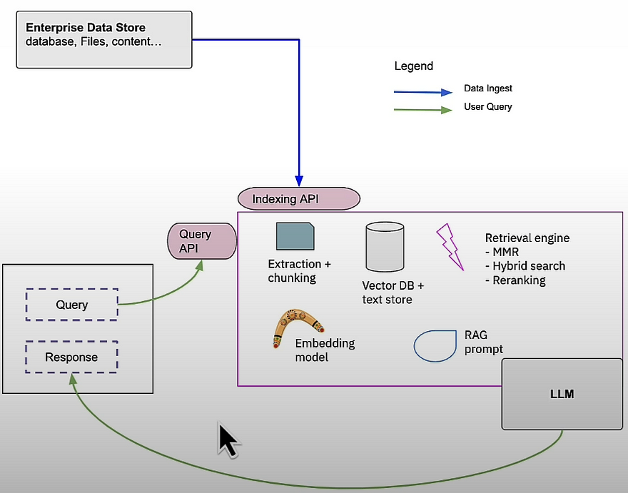
You can RAG on your own, using a framework like Langchain, or with a RAG-as-a-service platform like Vectara, which handles the majority of the heavy lifting for you.
Conclusion
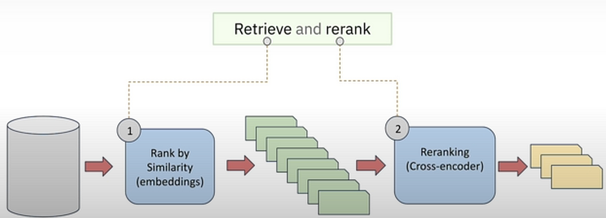
We conclude the essay by introducing the concept of a two-stage retrieval pipeline that leverages the strengths of embedding models and cross-encoders.
We discovered that vector pooling to obtain sentence embeddings did not work. We need to build a specialized model that trains on sentence pairs, specifically question-and-answer pairs. Sentence embedding models are faster but less accurate than cross encoders. A common practical approach is the two-stage retrieval approach, also known as Retrieve and Rerank, in which we use a sentence embedding model as a first-line filter to retrieve the top 100 matching documents, followed by a cross-encoder-based reranker to select one of the top ten best matches. This gives you a reasonable trade-off in terms of performance, latency, and accuracy. Several rankers are free source, with some commercial options from firms such as Vectara and Cohere.
We learned how to train a sentence embedding model. The contrastive loss function of the dual encoder. And how to leverage samples from a batch to create positive and negative examples. Embedding models are crucial components of any RAG implementation, whether used directly or as part of a two-stage retrieval workflow. We focus on embedding models; however, RAG includes alternative retrieval approaches to supplement neural search. One useful option is hybrid search, which combines neural search with classic keyword-based search. Another is the ability to filter facts by specific metadata values, such as including facts only if they are from publications by a certain author. MMR (Max Marginal Relevance) is another typical retrieval strategy that balances retrieval relevance with diversity of results.
For more check the following resources:
- Book by Jimmy Lin: https://arxiv.org/pdf/2010.06467
- Sentence Bert: https://arxiv.org/abs/1908.10084
- DPR Paper: https://arxiv.org/abs/2004.04906
- Reqa Paper: https://arxiv.org/pdf/1907.04780
- Vectara’s Boomerang Sentence Embedding Model: https://vectara.com/blog/introducing-boomerang-vectaras-new-and-improved-retrieval-model/
Resource
[1] Deeplearning.ai, (2024), Embedding Models: From Architecture to Implementation:
[https://learn.deeplearning.ai/courses/embedding-models-from-architecture-to-implementation/]

0 Comments