
“Tokenization is one of the really critical but often ignored and underappreciated aspects of the models we use. ”-Andrew NG.
This course focuses on improving and optimizing retrieval for RAG and search applications. You start by learning about how tokenization works in LLMs and embedding models, as well as how the tokenizer affects search quality. Tokenizers generate a sequence of numerical IDs of integers that represent tokens, which often correspond to words or sections of words in a text. There are several approaches of converting a text into a sequence of tokens. For example, a word tokenizer tokenizes sentences word for word, but a subword tokenizer tokenizes letters or character combinations.We'll learn about tokenization approaches including binary byte-pair encoding and unigram tokenization, as well as how token vocabulary affects search results, particularly for unusual characters like emoticons, typos, and numerical values.
The first step in optimizing your system is to evaluate the quality of its outputs. So, in this course, we'll learn how to use numerous quality measures to evaluate the quality of our search results. Vector databases employ specialized data structures to approximate the search for nearest neighbours. HNSW, which stands for Hierarchical Navigable, Small Words, is the most widely used, and it contains some options that allow you to decide how good the approximation. HNSW search is based on a multi-layer graph, similar to how a product is shipped via postal. The first layer brings you close enough to the state where mail should be delivered, the next layer locates the city, and as you go down the levels, you get closer.
We will look at how to balance the settings for building and searching the HNSW graph to achieve maximum speed and relevancy. If you have millions of vectors to search, storing, indexing, and searching can become time-consuming and inefficient. Assume you created a news analysis software that aggregates and summarizes all industry-related news. After chunking hundreds of articles published every day for a month, you could wind up with millions of vector embeddings. If you end up with 5 million vectors, OpenAI's Ada embedding model, which generates a vector with slightly more than 1500 dimensions, will require approximately 30 GB of RAM and will continue to expand each month. This is where quantification approaches come in.
Using the strategies taught in this course, you can reduce the memory required for your vector search by up to 64 times. You'll master three major quantization approaches. The first step is product quantization. This assigns subsectors to the nearest centroid, which either reduces memory consumption or increases indexing time. The second step is scalar quantization, which converts each float value to a 1-byte integer. This considerably reduces memory and speeds up indexing and search operations, but it reduces precision marginally. The third type of quantization is binary quantization, which converts float values to Boolean values, dramatically increasing memory use and search performance at the expense of precision.
Embedding models
Let's look at how embedding models work internally. We'll look into how an embedding model converts texts into vectors using various layers. If you train your embedding model on scientific papers and then try to use it on Tweets, the accuracy will suffer. The embedding model transforms a text into a fixed-dimensionality vector, allowing us to compare the distance between any two publications and evaluate similarity.
Embedding models do not work with text directly. Instead, they require a further procedure known as tokenization to divide it into smaller bits.
The transformer architecture consists of an encoder and a decoder. Embedding models only use encoder transformer designs. The model's inputs are mapped to input embeddings in embedding models, and each input has a matching embedding that was learned during training. This means transformers can only process the input symbols they were educated on. The embedding models can only work with text units found in the training data. Tokenizers generate a series of numerical IDs that correspond to the tokens seen in a given text. These IDs form a contract between the tokenizer and the voting model. As a result, once the training is completed, we cannot easily switch the components due to the ID.
The most basic way is to let the model function directly on a character or byte level, resulting in a narrow vocabulary and increased ambiguity. The amount of the vocabulary will also affect how many input embeddings the model learns. However, because each character can appear in a variety of contexts, the embedding is meaningless. The network parameters must understand the association between the letters and deduce what the sequence signifies.
In contrast to character-based tokenization, we may utilize word tokens, with each word receiving its own identifier, and the model learning additional embeddings to cover them all. This translates to greater training data and time spent on training. Furthermore, we would be unable to represent any unknown word as a series of tokens because we would only cover complete words. That would never occur with character or byte-level tokenization. This concept ignores the reality that language has structure, and some words may share common elements that carry meaning.
Subword-level tokenization appears to be a compromise between these two main approaches. For example, words with the same root form have similar meanings. This strategy is based on natural language processing, such as stemming or lemmatization. It can be trained using statistical methods. Example: walk|er|walk|ed. However, in other languages, it may do poorly.
Let us follow the process of transforming text into embeddings step by step. First, we split into tokens with the chosen tokenizer. The tokenizer generates a series of token IDs and passes them to the model. The model converts each token ID into a learnt input embedding. The initial step in the transformer is a lookup table. It'll be fascinating to see how its input embeddings change with different texts.
import warnings
warnings.filterwarnings('ignore')
from sentence_transformers import SentenceTransformer

model = SentenceTransformer("all-MiniLM-L6-v2")
print(model)
This model includes a transformer, a meaning pooling layer, and normalizing. This output obscures the tokenizer component, which is also significant. You can tokenize the text by calling the model's tokenized method. It may accept many texts at once and requires a list of strings.
tokenized_data = model.tokenize(["walker walked a long walk"])
print(tokenized_data)
Using a list of input IDs is not the most simple or user-friendly method of evaluating how the input text was divided into chunks. To get a list of tokens, send a list of appropriate IDs to the model's tokenizer's convert IDs to tokens method.
print(model.tokenizer.convert_ids_to_tokens(tokenized_data["input_ids"][0]))
Each word in our example corresponds to a token learned by the tokenizer. There are also several technical tokens with square brackets. CLS and SEP initiate and terminate each sequence.
# Transformer consists of multiple stack modules. Tokens are an input
# of the first one, so we can ignore the rest.
first_module = model._first_module()
print(first_module.auto_model)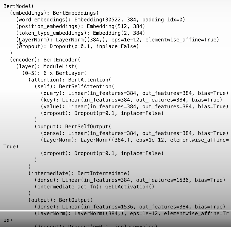
# input token embeddings
embeddings = first_module.auto_model.embeddings
print(embeddings)
Word embeddings capture the meaning of the words.
import torch
import plotly.express as px

device = torch.device("mps" if torch.has_mps else "cpu")  # Use MPS for Apple, CUDA for others, or fallback to CPU

first_sentence = "vector search optimization"
second_sentence = "we learn to apply vector search optimization"

with torch.no_grad():
    # Tokenize both texts
    first_tokens = model.tokenize([first_sentence])
    second_tokens = model.tokenize([second_sentence])

    # Get the corresponding embeddings
    first_embeddings = embeddings.word_embeddings(
        first_tokens["input_ids"].to(device)
    )
    second_embeddings = embeddings.word_embeddings(
        second_tokens["input_ids"].to(device)
    )

first_embeddings.shape, second_embeddings.shape

from sentence_transformers import util

distances = util.cos_sim(
    first_embeddings.squeeze(),
    second_embeddings.squeeze()
).cpu().numpy() # Move the tensor to the CPU and convert to a NumPy array

px.imshow(
    distances,
    x=model.tokenizer.convert_ids_to_tokens(
        second_tokens["input_ids"][0]
    ),
    y=model.tokenizer.convert_ids_to_tokens(
        first_tokens["input_ids"][0]
    ),
    text_auto=True,
)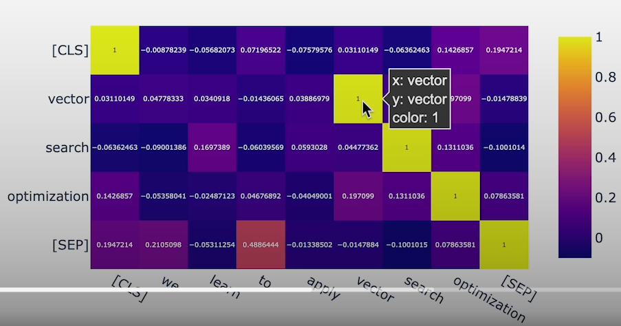
The succession of word embeddings has no positional information. To fix this, we employ position embeddings, resulting in a slightly updated set of token embeddings that should capture the relationships between tokens throughout the text. Positional encodings are often created using a sine function. Once both input token embeddings and positional encodings have been added, we run them through a series of stacked layers, each of which is taken up by the input embeddings and produces some output embeddings. Internally, each of these modules uses attention techniques to detect the links between input embeddings, hence this is where all cross-token information is stored.
We have 3 groups of tokens in our vocabulary. Technical tokens that are specific to the model, subword tokens with ##prefixes and prefixes and words starting with anything except ##.
# visualizing the input embeddings
token_embeddings = first_module.auto_model \
    .embeddings \
    .word_embeddings \
    .weight \
    .detach() \
    .cpu() \
    .numpy()
token_embeddings.shape

import random

vocabulary = first_module.tokenizer.get_vocab()
sorted_vocabulary = sorted(
    vocabulary.items(),
    key=lambda x: x[1],  # uses the value of the dictionary entry
)
sorted_tokens = [token for token, _ in sorted_vocabulary]
random.choices(sorted_tokens, k=100)

from sklearn.manifold import TSNE

tsne = TSNE(n_components=2, metric="cosine", random_state=42)
tsne_embeddings_2d = tsne.fit_transform(token_embeddings)
tsne_embeddings_2d.shape

token_colors = []
for token in sorted_tokens:
    if token[0] == "[" and token[-1] == "]":
        token_colors.append("red")
    elif token.startswith("##"):
        token_colors.append("blue")
    else:
        token_colors.append("green")

import plotly.graph_objs as go

scatter = go.Scattergl(
    x=tsne_embeddings_2d[:, 0],
    y=tsne_embeddings_2d[:, 1],
    text=sorted_tokens,
    marker=dict(color=token_colors, size=3),
    mode="markers",
    name="Token embeddings",
)

fig = go.FigureWidget(
    data=[scatter],
    layout=dict(
        width=600,
        height=900,
        margin=dict(l=0, r=0),
    )
)

fig.show()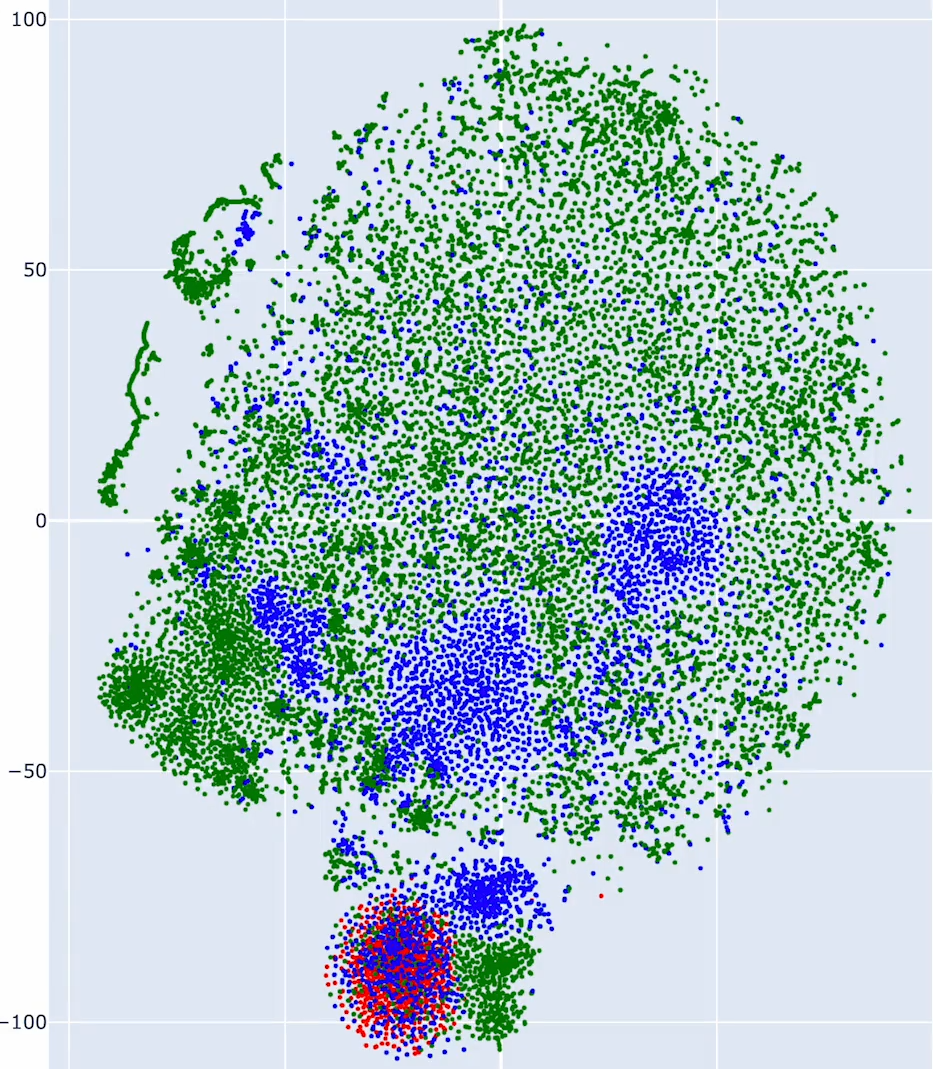
# output token embeddings
output_embedding = model.encode(["walker walked a long walk"])
output_embedding.shape

output_token_embeddings = model.encode(
    ["walker walked a long walk"],
    output_value="token_embeddings"
)
output_token_embeddings[0].shape

first_sentence = "vector search optimization"
second_sentence = "we learn to apply vector search optimization"

with torch.no_grad():
    first_tokens = model.tokenize([first_sentence])
    second_tokens = model.tokenize([second_sentence])

    first_embeddings = model.encode(
        [first_sentence],
        output_value="token_embeddings"
    )
    second_embeddings = model.encode(
        [second_sentence],
        output_value="token_embeddings"
    )

distances = util.cos_sim(
    first_embeddings[0],
    second_embeddings[0]
)

px.imshow(
    distances.cpu().numpy(),  # Move the tensor to CPU and convert to a NumPy array
    x=model.tokenizer.convert_ids_to_tokens(
        second_tokens["input_ids"][0]
    ),
    y=model.tokenizer.convert_ids_to_tokens(
        first_tokens["input_ids"][0]
    ),
    text_auto=True,
)
Role of the Tokenizers
In this session, we will train numerous tokenizers. Because they determine how the transformer model interprets incoming text, they deserve special attention. There are various tokenizer algorithms. Tokenizer training, unlike LLM training, is completely deterministic and dependent on the statistics of the input data.
Various models use different tokenization approaches. OpenAI chooses byte-per-encoding, while Cohere English V3 prefers WordPiece, Cohere Multilingual V3 prefers Unigram, and Sentence Transformer all-MiniLM-L6-V2 utilizes WordPiece. The vocabulary size is a parameter that must be chosen at the outset, and it is typically at least 30k tokens, while for multilingual models it may be significantly higher, such as 200k tokens.
Check the most popular tokenization algorithms and see how they split the text.
BPE (Byte Pair Encoding)
BPE is a typical choice for LLMs. In BPE, words are often separated by whitespace characters and then divided into characters or bytes. New tokens are repeatedly formed by combining two tokens that are frequently placed adjacent to one other. We select the most common portion and add it to the vocabulary, but we do not remove the tokens required to construct it.A tokenizer is a generic component that takes a tokenization model as an input. It also allows us to specify the tokenization that will be performed on each input text before we begin tokenizing it. Whiespace pre-tokenization aids in the breakdown of text into words. The final thing you'll set is the trainer object and the size of a target vocabulary.
You will now train the tokenizer using a Python iterator by feeding the training set to a corresponding trainer instance. Then you can check your vocabulary to see what tokens you've learnt. The training process is iterative, thus just verifying their IDs reveals the sequence in which new tokens were added to the lexicon.
training_data = [
    "walker walked a long walk",
]

from tokenizers.trainers import BpeTrainer
from tokenizers.models import BPE
from tokenizers import Tokenizer
from tokenizers.pre_tokenizers import Whitespace

bpe_tokenizer = Tokenizer(BPE())
bpe_tokenizer.pre_tokenizer = Whitespace()
bpe_trainer = BpeTrainer(vocab_size=14) # Generally few thousand but for demo it is 14

bpe_tokenizer.train_from_iterator(training_data, bpe_trainer)

bpe_tokenizer.get_vocab()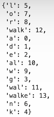
bpe_tokenizer.encode("walker walked a long walk").tokens
# ['walke', 'r', 'walke', 'd', 'a', 'l', 'o', 'n', 'g', 'walk']

bpe_tokenizer.encode("wlk").ids
# [9, 5, 4]

bpe_tokenizer.encode("wlk").tokens
# ['w', 'l', 'k']

bpe_tokenizer.encode("she walked").tokens # s and h never occured in training phase so they are omitted
# ['e', 'walke', 'd']
WordPiece
Similar to BPE and commonly used in embedding models. WordPiece separates first and middle letters by attaching a double hash prefix. The typical approach is to study words, prefixes, and suffixes independently.
The training procedure begins with a vocabulary composed of each word's letters and the middle letters of words preceded with a double hash. The algorithm then iteratively merges the token pairings, but does so based on the score, which differs from BPE. We no longer select the most common portion, but rather assess how frequently these two tokens appear in different situations. When we calculate the scores for each pair of tokens in the first iteration, it is clear that if two tokens always appear next to each other, they will be chosen for merge. Similarly to BPE, we add additional tokens iteratively. When the necessary token size is reached, the procedure will stop.
score(u,v) = frequency(uv) / (frequency(u)*frequency(v))
Since WordPiece adds all the single letters and middle letters as separate tokens we usually need a bigger vocabulary to capture these regularities.
from real_wordpiece.trainer import RealWordPieceTrainer
from tokenizers.models import WordPiece

real_wordpiece_tokenizer = Tokenizer(WordPiece())
real_wordpiece_tokenizer.pre_tokenizer = Whitespace()

real_wordpiece_trainer = RealWordPieceTrainer(
    vocab_size=27,
)

real_wordpiece_trainer.train_tokenizer(
    training_data, real_wordpiece_tokenizer
)
real_wordpiece_tokenizer.get_vocab()

real_wordpiece_tokenizer.encode("walker walked a long walk").tokens

real_wordpiece_tokenizer.encode("wlk").tokens

# The following line will produce an error because it contains unknown characters. Please uncomment the line and run it to see the error.
# real_wordpiece_tokenizer.encode("she walked").tokens
HuggingFace WordPiece and special tokens
from tokenizers.trainers import WordPieceTrainer
unk_token = "[UNK]"
wordpiece_model = WordPiece(unk_token=unk_token)
wordpiece_tokenizer = Tokenizer(wordpiece_model)
wordpiece_tokenizer.pre_tokenizer = Whitespace()
wordpiece_trainer = WordPieceTrainer(
    vocab_size=28,
    special_tokens=[unk_token]
)

wordpiece_tokenizer.train_from_iterator(
    training_data,
    wordpiece_trainer
)
wordpiece_tokenizer.get_vocab()

wordpiece_tokenizer.encode("walker walked a long walk").tokens
wordpiece_tokenizer.encode("wlk").tokens
wordpiece_tokenizer.encode("she walked").tokens
Unigram

Unlike BPE and WordPiece, Unigram begins with a large vocabulary that is reduced over the training process. Unigram begins with a large vocabulary and subsequently removes some tokens based on calculated loss. The basic vocabulary allows you to tokenize a single word in a variety of ways.

The list of all potential tokenizations is required to determine the loss during the Unigram training process. At each iteration, the algorithm calculates how much the aggregate loss would increase if a certain token was eliminated, and then searches for the tokens that would increase it the least. Probabilities are established by the token frequencies.
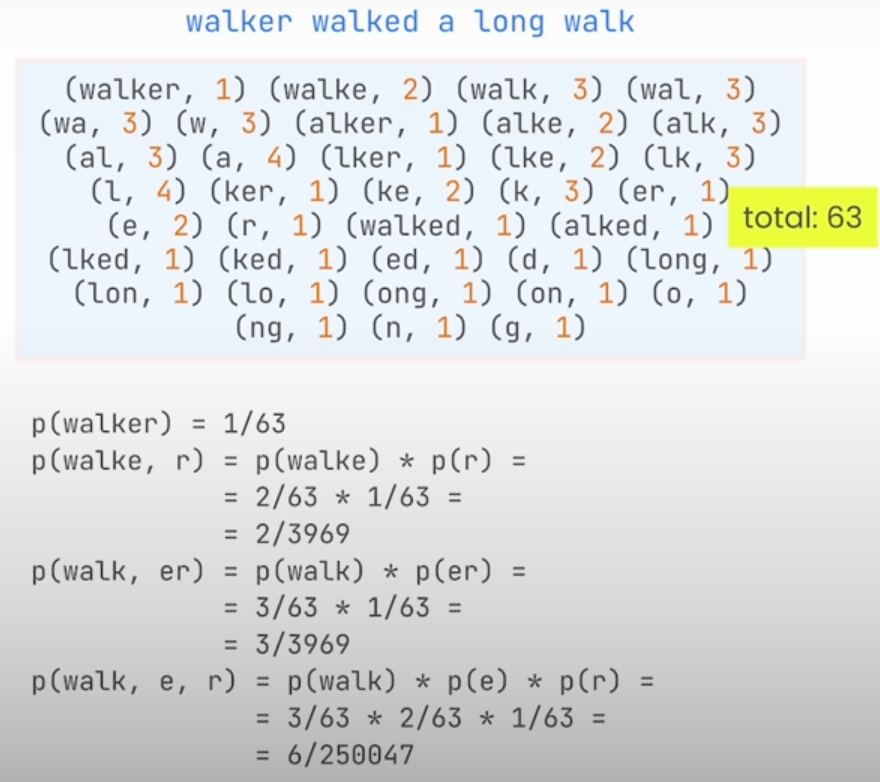
There are 63 instances of the tokens in all. That is, we can calculate the chance of a specific tokenization as a function of the frequencies of all tokens utilized. Even in this simple case, the number of tokenizations to consider is very large. Unigram training will determine how deleting each token will affect the loss and then select the one that can be deleted with the least influence on the loss. Analyzing each phase of the unigram training process would take a large number of computations. Unigram removes a few tokens at each phase and simply ensures that the vocabulary size does not exceed the intended limit. We can see that common prefixes were discovered to be crucial, therefore the hope is that our tokenization can capture the meaning correctly. We only have the base alphabet and the common prefixes of the words, no double-letter tokens.
from tokenizers.trainers import UnigramTrainer
from tokenizers.models import Unigram

unigram_tokenizer = Tokenizer(Unigram())
unigram_tokenizer.pre_tokenizer = Whitespace()
unigram_trainer = UnigramTrainer(
    vocab_size=14,
    special_tokens=[unk_token],
    unk_token=unk_token,
)

unigram_tokenizer.train_from_iterator(training_data, unigram_trainer)
unigram_tokenizer.get_vocab()

unigram_tokenizer.encode("walker walked a long walk").tokens

unigram_tokenizer.encode("wlk").tokens

unigram_tokenizer.encode("she walked").tokens
# ['sh', 'e', 'walke', 'd']

unigram_tokenizer.encode("she walked").ids
SentencePiece is simply an implementation of the same tokenization procedures, plus one additional text-related assumption, rather than a new approach. SentencePiece does not text with white spaces, but instead handles them as any other character. This allows it to function with languages that don't use them as separators. Internally, SentencePiece builds its vocabulary using byte per encoding or Unigram. SentencePiece allows you to create tokens that span multiple words, including whitespaces. This method is important whether you're using a code tokenizer like Python or employing unique names like San Francisco or Real Madrid.
Practical implications of the tokenization
Vector search alone may require revision. You will focus on some of the most prevalent difficulties and learn how to efficiently address them with vector databases.
If a specific token appears in multiple situations in the training data, it has no apparent meaning. This is especially true for subword tokens, which frequently appear in various contexts.
The BPE paper shows that the fewer tokens used to cover the test set, the better the results may be.
Typos, dates, numerical quantities, and emoticons are all potential stumbling blocks. OpenAI does this via byte-level encoding.
from sentence_transformers import SentenceTransformer, util

sbert_model = SentenceTransformer("all-MiniLM-L6-v2")
out_vector = sbert_model.encode("Vector search optimization")
out_vector.shape

sbert_tokenizer = sbert_model.tokenizer._tokenizer
sbert_tokenizer

sbert_tokenizer.encode("I feel 😊").tokens
# ['[CLS]', 'i', 'feel', '[UNK]', '[SEP]']

sbert_tokenizer.encode("I feel happy").tokens

sbert_tokenizer.encode("Broadcom BCM2712").tokens
#['[CLS]', 'broad', '##com', 'bc', '##m', '##27', '##12', '[SEP]']

sentences = [
    "Great accommodation",
    "Great acommodation", # because of typo, tokenization is different
]
for sentence in sentences:
    print(sbert_tokenizer.encode(sentence).tokens)

sentences = [
    "This shirt costs $55.",
    "This shirt costs fifty five dollars.",
    "This shirt costs $50.",
    "This shirt costs $559.",
    "This shirt has a 10% discount from $60.",
]
for sentence in sentences:
    print(sbert_tokenizer.encode(sentence).tokens)

sentences = [
    "16th February 2024",
    "2024-02-16",
    "17th February 2024",
    "18th February 2024",
    "19th February 2024",
    "20th February 2024",
    "15th February 2024",
]
for sentence in sentences:
    print(sbert_tokenizer.encode(sentence).tokens)

# Implications on semantic similarity

import plotly.express as px

sentences = [
    "I feel 😊",
    "I feel happy",
    "I feel 🙁",
    "I feel sad",
]
embeddings = sbert_model.encode(sentences)
cosine_scores = util.cos_sim(embeddings, embeddings)

px.imshow(
    cosine_scores,
    x=sentences,
    y=sentences,
    text_auto=True,
)

# Typos
sentences = [
    "Great accommodation",
    "Great acommodation",
]
embeddings = sbert_model.encode(sentences)
cosine_scores = util.cos_sim(embeddings, embeddings)
px.imshow(
    cosine_scores,
    x=sentences,
    y=sentences,
    text_auto=True,
)

# Numerical values and datetime

sentences = [
    "This shirt costs $55.",
    "This shirt costs fifty five dollars.",
    "This shirt costs $50.",
    "This shirt costs $559.",
    "This shirt has a 10% discount from $60.",
]
embeddings = sbert_model.encode(sentences)
cosine_scores = util.cos_sim(embeddings, embeddings)
fig = px.imshow(
    cosine_scores,
    x=sentences,
    y=sentences,
    text_auto=True,
)
fig.update_xaxes(tickangle=-30)

sentences = [
    "16th February 2024",
    "2024-02-16",
    "17th February 2024",
    "18th February 2024",
    "19th February 2024",
    "20th February 2024",
    "15th February 2024",
]
embeddings = sbert_model.encode(sentences)
cosine_scores = util.cos_sim(embeddings, embeddings)
fig = px.imshow(
    cosine_scores,
    x=sentences,
    y=sentences,
    text_auto=True,
)
fig.update_layout(
    xaxis={"type": "category"},
    yaxis={"type": "category"}
)
fig.update_xaxes(tickangle=-30)

# Impact on different models

import tiktoken

openai_tokenizer = tiktoken.encoding_for_model("text-embedding-3-large")
openai_tokenizer.n_vocab
token_ids = openai_tokenizer.encode("I feel 😊")
openai_tokenizer.decode_tokens_bytes(token_ids)
token_ids = openai_tokenizer.encode("I feel happy")
openai_tokenizer.decode_tokens_bytes(token_ids)
token_ids = openai_tokenizer.encode("Broadcom BCM2712")
openai_tokenizer.decode_tokens_bytes(token_ids)
sentences = [
    "Great accommodation",
    "Great acommodation",
]
for sentence in sentences:
    token_ids = openai_tokenizer.encode(sentence)
    print(openai_tokenizer.decode_tokens_bytes(token_ids))
sentences = [
    "This shirt costs $55.",
    "This shirt costs fifty five dollars.",
    "This shirt costs $50.",
    "This shirt costs $559.",
    "This shirt has a 10% discount from $60.",
]
for sentence in sentences:
    token_ids = openai_tokenizer.encode(sentence)
    print(openai_tokenizer.decode_tokens_bytes(token_ids))
sentences = [
    "16th February 2024",
    "2024-02-16",
    "17th February 2024",
    "18th February 2024",
    "19th February 2024",
    "20th February 2024",
    "15th February 2024",
]
for sentence in sentences:
    token_ids = openai_tokenizer.encode(sentence)
    print(openai_tokenizer.decode_tokens_bytes(token_ids))

# Vector similarity
from openai import OpenAI
from helper import get_openai_api_key

openai_client = OpenAI(api_key=get_openai_api_key())
sentences = [
    "I feel 😊",
    "I feel happy",
    "I feel 🙁",
    "I feel sad",
]
embeddings = [
    embedding.embedding
    for embedding in openai_client.embeddings.create(
        input=sentences, model="text-embedding-3-large"
    ).data
]
cosine_scores = util.cos_sim(embeddings, embeddings)
px.imshow(
    cosine_scores,
    x=sentences,
    y=sentences,
    text_auto=True,
)
sentences = [
    "Great accommodation",
    "Great acommodation",
]
embeddings = [
    embedding.embedding
    for embedding in openai_client.embeddings.create(
        input=sentences, model="text-embedding-3-large"
    ).data
]
cosine_scores = util.cos_sim(embeddings, embeddings)
fig = px.imshow(
    cosine_scores,
    x=sentences,
    y=sentences,
    text_auto=True,
)
fig.update_xaxes(tickangle=-30)
sentences = [
    "This shirt costs $55.",
    "This shirt costs fifty five dollars.",
    "This shirt costs $50.",
    "This shirt costs $559.",
    "This shirt has a 10% discount from $60.",
]
embeddings = [
    embedding.embedding
    for embedding in openai_client.embeddings.create(
        input=sentences, model="text-embedding-3-large"
    ).data
]
cosine_scores = util.cos_sim(embeddings, embeddings)
fig = px.imshow(
    cosine_scores,
    x=sentences,
    y=sentences,
    text_auto=True,
)
fig.update_xaxes(tickangle=-30)
sentences = [
    "16th February 2024",
    "2024-02-16",
    "17th February 2024",
    "18th February 2024",
    "19th February 2024",
    "20th February 2024",
    "15th February 2024",
]
embeddings = [
    embedding.embedding
    for embedding in openai_client.embeddings.create(
        input=sentences, model="text-embedding-3-large"
    ).data
]
cosine_scores = util.cos_sim(embeddings, embeddings)

fig = px.imshow(
    cosine_scores,
    x=sentences,
    y=sentences,
    text_auto=True,
)
fig.update_layout(
    xaxis={"type": "category"},
    yaxis={"type": "category"}
)
fig.update_xaxes(tickangle=-30)

# Vector search in practice
from qdrant_client import QdrantClient, models
client = QdrantClient("http://localhost:6333")
client.get_collections()

examples = [
    ("Sleeveless maxi dress with a V-neckline and wrap front."
     "Comes with a tie belt at the waist.", 29.95),
    ("Slim-fit jeans in washed stretch denim with a button fly "
     "and tapered legs.", 39.99),
    ("Double-breasted blazer in textured-weave fabric with peak "
     "lapels and front flap pockets.", 59.50),
    ("Lightweight bomber jacket with ribbed cuffs, a baseball collar, "
     "and zip front closure.", 45.00),
    ("Chunky knit sweater with dropped shoulders and ribbed trim around "
     "the neck, cuffs, and hem.", 25.99),
    ("Tailored trousers in a smooth woven fabric with a concealed "
     "hook-and-eye closure and welt back pockets.", 34.99),
    ("Classic trench coat with adjustable belt, storm flap, and button "
     "front closure.", 79.90),
    ("High-rise pencil skirt in a stretch fabric with a hidden rear zip "
     "and back slit.", 22.99),
    ("Athletic-fit polo shirt in moisture-wicking fabric with a ribbed "
     "collar and two-button placket.", 19.95),
    ("Soft flannel pajama set with long sleeves, matching pants, and a "
     "comfortable elastic waistband.", 32.00),
    ("Quilted puffer jacket with a detachable hood and zippered side "
     "pockets.", 48.99),
    ("Cropped denim jacket with distressed details and button-flap chest "
     "pockets.", 36.50),
    ("Fitted bodysuit with a scoop neckline and snap-button closure at "
     "the bottom.", 15.99),
    ("Lightly padded parka with a faux fur-lined hood, drawstring waist, "
     "and snap front pockets.", 69.95),
    ("Mesh panel sports leggings with a high waist and reflective details "
     "for nighttime visibility.", 27.99),
    ("Button-up cardigan in a soft knit with long sleeves and ribbed "
     "trim.", 24.50),
    ("Leather moto jacket with zippered cuffs, a notched collar, and "
     "asymmetrical zip closure.", 95.00),
    ("Velvet slip dress with a lace trim neckline and adjustable "
     "spaghetti straps.", 31.99),
    ("Cargo shorts with multiple pockets and a durable belt loop "
     "waistband.", 22.95),
    ("Wide-leg palazzo pants with a high-rise fit and side zip "
     "closure.", 38.99),
    ("Graphic print tee featuring an original artwork design and classic "
     "crew neck.", 14.99),
    ("Boho-style maxi skirt with an elastic waistband and tiered ruffle "
     "detailing.", 33.50),
    ("Men's linen shirt with a Mandarin collar and buttoned chest "
     "pocket.", 29.95),
    ("Cable knit beanie with a fold-over cuff and soft fleece "
     "lining.", 12.99),
    ("Sequin cocktail dress with a plunging V-neck and bodycon "
     "fit.", 49.99),
]

client.delete_collection("clothes")
client.create_collection(
    "clothes",
    vectors_config=models.VectorParams(
        size=384,
        distance=models.Distance.COSINE,
    )
)

import uuid

client.upsert(
    "clothes",
    points=[
        models.PointStruct(
            id=uuid.uuid4().hex,
            vector=sbert_model.encode(description),
            payload={"description": description, "price": price},
        )
        for description, price in examples
    ]
)

client.search(
    "clothes",
    query_vector=sbert_model.encode("for cold weather"),
    with_payload=True,
    limit=3,
)

# Vector search with additional constraints
client.search(
    "clothes",
    query_vector=sbert_model.encode("for cold weather under $40"),
    with_payload=True,
    limit=3,
)
client.create_payload_index(
    "clothes",
    field_name="price",
    field_schema=models.PayloadSchemaType.FLOAT,
)
client.search(
    "clothes",
    query_vector=sbert_model.encode("for cold weather"),
    with_payload=True,
    limit=3,
    query_filter=models.Filter(
        must=[
            models.FieldCondition(
                key="price",
                range=models.Range(
                    lte=40.0,
                )
            )
        ]
    )
)
Measuring Search Relevance
We will learn the tools and most commonly used metrics for information retrieval in RAG. You can’t improve what you can’t measure. Measuring the quality of system outputs is the first thing to do in optimization.
First, we build a ground truth dataset that has pairs including queries with the best matching documents. Building it requires a lot of human labour. The different items might be more relevant for different groups of people even if the query is the same.
There are 2 typical ways of annotating the relevance of a document-given query. Binary (item is relevant or not) or numerical (relevance is expressed as an item).
import pandas as pd

products_df = pd.read_csv(
    "shared_data/WANDS/product.csv",
    sep="\t",
    index_col="product_id",
    keep_default_na=False,  # some products do not have a description
)
products_df.head()
num_products = 5000
from sentence_transformers import SentenceTransformer

model = SentenceTransformer("all-MiniLM-L6-v2")

product_name_embeddings = model.encode(
    products_df["product_name"][0:num_products].tolist()
)
product_name_embeddings.shape
product_description_embeddings = model.encode(
    products_df["product_description"][0:num_products].tolist()
)
product_description_embeddings.shape
# Building the collection
from qdrant_client import QdrantClient, models

client = QdrantClient("http://localhost:6333")
client.delete_collection("wands-products")
client.create_collection(
    collection_name="wands-products",
    vectors_config={
        "product_name": models.VectorParams(
            size=384,
            distance=models.Distance.COSINE,
        ),
        "product_description": models.VectorParams(
            size=384,
            distance=models.Distance.COSINE,
        ),
    },
    optimizers_config=models.OptimizersConfigDiff(
        default_segment_number=2,
        indexing_threshold=1000,
    ),
)
client.upload_collection(
    collection_name="wands-products",
    vectors={
        "product_name": product_name_embeddings,
        "product_description": product_description_embeddings,
    },
    payload=products_df.to_dict(orient="records"),
    ids=products_df.index.tolist(),
    batch_size=64,
)
client.count("wands-products")
import time

time.sleep(1.0)
collection = client.get_collection("wands-products")
while collection.status != models.CollectionStatus.GREEN:
    time.sleep(1.0)
    collection = client.get_collection("wands-products")

collection
# Test queries
queries_df = pd.read_csv(
    "shared_data/WANDS/query.csv",
    sep="\t",
    index_col="query_id",
)
queries_df.head()
# Ground truth
labels_df = pd.read_csv(
    "shared_data/WANDS/label.csv",
    sep="\t",
)
labels_df.sample(n=5)
relevancy_scores = {
    "Exact": 10,
    "Partial": 5,
    "Irrelevant": 0,
}

labels_df["score"] = labels_df["label"].map(relevancy_scores.get)
labels_df["query_id"] = labels_df["query_id"].map(lambda x: f"query_{x}")
labels_df["product_id"] = labels_df["product_id"].map(lambda x: f"doc_{x}")
labels_df.sample(n=5)
Search engines identify the N documents that are most relevant to a given query. For vector search, the distance function is an obvious choice for a relevancy metric. The outcomes are ranked according to their score. Quality metrics could be loosely classified into three categories:
- Relevance-based
- Ranking-related metrics.
- Score related metrics.
Relevancy Based Metrics
The percentage of relevant papers in the first k results. Precision@k is a commonly used method for calculating the quality of the research system. This metric calculates the proportion of relevant items among the top k results returned by our system. If we return fewer than K relevant pages, obtaining a 100% score may be unachievable, but it is still a useful method for comparing different search pipelines. Precision at K is calculated per query y, and we typically give the average precision at K for all queries in the ground truth dataset.
precision@k = |relevant documents in the top k results| / k
Similarly, recall@k determines how many relevant documents we can return in the top k results. Perfectly, we would return 100% of them, however this may be difficult if there are more than k relevant documents per query.
recall@k = |relevant documents in the top k results| / |all relevant documents|
It’s common to present both precision and recall together.
The order of the document is important. This group includes the regularly used measure Mean Reciprocal Rank. It is based on the location of the first relevant item in the search results. It is used to assess a system's ability to produce highly relevant results as quickly as possible. It just evaluates the location of the most relevant one. The first place in Google results receives the most clicks.
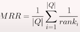
rank_i is the position of the first relevant item.
Score-based measures are also widely employed. Discounted Cumulative Gain is one example. It assesses the overall relevance of the returned documents while also addressing the issue of diminishing relevance of things further down the results list. It lends more weight to papers that appear earlier in the list, indicating the decreasing relevance via a logarithmic scale for the position.
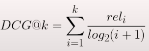
There is an alternative formulation emphasizing the relevance score.

If we have the relevancy scores in our ground truth, we can calculate the Ideal Discounted Cumulative Gain, with the same formula as DCG.

Ranx
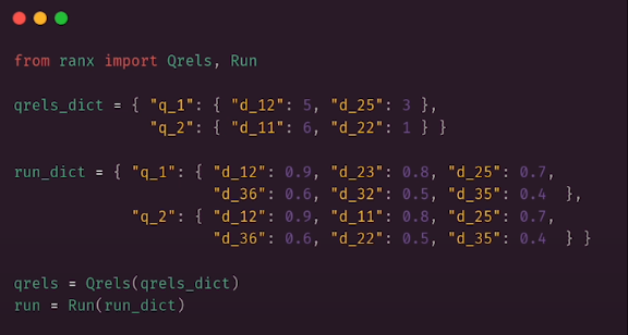
Ranx is a library for writing metrics. There are two major concepts. Qrels, or query relevance judgments (ground truths), are an output of the retrieval system. Generally, for each query, we established a group of documents and their significance. In the case of Qrels, the significance is an integer, with larger values indicating a stronger match. Convert all of the queries into embeddings so that they may be used in the assessments. Ranx requires a run object, which describes the results of a certain query. Each retrieved document should receive the score assigned by the search process. You will do it twice, first by looking for the product's name. We will create a dictionary that will store the run object data. To accomplish this, we need to iterate on run queries and then run a search operation on the collection we created before. This dictionary is converted to a Run object. Finally, we compare both search pipelines. Ranx allows passing metrics as strings.
# ranx
from ranx import Qrels

qrels = Qrels.from_df(
    labels_df.astype({"query_id": "str", "product_id": "str"}),
    q_id_col="query_id",
    doc_id_col="product_id",
    score_col="score",
)

# Running all the queries
queries_df["query_embedding"] = model.encode(
    queries_df["query"].tolist()
).tolist()
queries_df.sample(n=5)
from collections import defaultdict

name_run_dict = defaultdict(dict)
for id, row in queries_df.iterrows():
    query_id = f"query_{id}"

    results = client.search(
        collection_name="wands-products",
        query_vector=models.NamedVector(
            name="product_name",
            vector=row["query_embedding"]
        ),
        with_vectors=False,
        with_payload=False,
        limit=100,
    )

    for point in results:
        document_id = f"doc_{point.id}"
        name_run_dict[query_id][document_id] = point.score

name_run_dict
from ranx import Run

product_name_run = Run(name_run_dict, name="product_name")
description_run_dict = defaultdict(dict)
for id, row in queries_df.iterrows():
    query_id = f"query_{id}"

    results = client.search(
        collection_name="wands-products",
        query_vector=models.NamedVector(
            name="product_description",
            vector=row["query_embedding"]
        ),
        with_vectors=False,
        with_payload=False,
        limit=100,
    )

    for point in results:
        document_id = f"doc_{point.id}"
        description_run_dict[query_id][document_id] = point.score

product_description_run = Run(
    description_run_dict,
    name="product_description"
)
from ranx import compare

compare(
    qrels=qrels,
    runs=[
        product_name_run,
        product_description_run
    ],
    metrics=[
        "precision@10",
        "recall@10",
        "mrr@10",
        "dcg@10",
        "ndcg@10",
    ],
)
All indicators indicate that the product name is a better option for semantic search.
Retrieval Augmented Generation is all about expanding prompts with relevant context so that the LLM may formulate the correct response. If we flood our prompts with unnecessary information, they will be ineffective. However, the entire process will fail if our search mechanism is unable to give the LLM with any significant results. That is why it is critical to do thorough testing.
Optimizing HNSW search
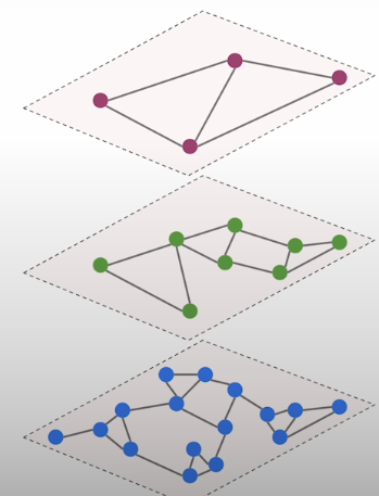
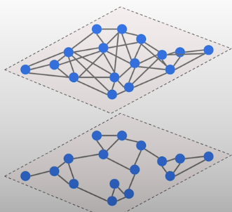
A quick overview of HNSW, the cornerstone of vector databases that enables efficient closest neighbor searches. There are some ways in which we can influence how effectively this approximation works. The hierarchically navigable Small Words is a multi-layer graph that simulates closest neighbor search. It connects vectors as nodes based on their similarity. As a result, the similarity measure must be determined ahead of time. A multilayer network of vectors in which connections are formed between the nearest locations. This data structure creates numerous layered graphs, the top one being the most sparse. This one only contains a small portion of all vectors. Each subsequent layer contains more and more, but the rule is that all the vectors from the previous layer are likewise present in the current layer. The bottom layer is dense as it contains all the vectors we have.
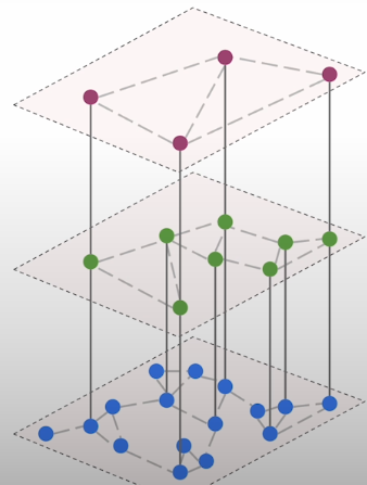
Aside from the similarity-based edges, there are internal layer connections that allow us to navigate between levels. They are generated between the same vectors, but at separate layers. HNSW has two parameters that we can change. The first one, M, specifies how many edges we build per node. Increasing this parameter's value should enhance approximation quality, but it will not address any issues with your embedding model. If your representations are simply too weak, you cannot expect ANN search to deduce the semantics of the data magically. Higher M numbers will simply move you closer to the exact k nearest neighbour search. However, adjusting this setting may also help with latency. In some circumstances, quality can be sacrificed.
The most common operation performed using the HNSW graph is searching. When we receive a query or want to add a new point to the graph, we begin with the top layer. When we receive a query, it is vectorized using the same embedding model and treated as an actual query. The search action begins at the top layer. Here, the algorithm locates the ef nearest points. Ef is the second metric to consider. In our example, its value was set to two, which is how many points we chose in the first layer. If we choose more options, we would obtain better outcomes, but the process would take longer.
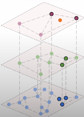
The points selected in the top layer are subsequently selected in the layer below via the intra-layer edges. We do not traverse all of the points here, but rather concentrate on the direct neighbours of the points chosen in the previous phase. Again, we select the closest matches, and the process continues. Repeat the process until we reach the bottom layer. Each time, we just look at the previously picked spots and their direct neighbors. That effectively reduces the scope of the search. In the last layer, we select the top k elements, and these vectors become the most relevant documents to return.
from qdrant_client import QdrantClient, models

client = QdrantClient("http://localhost:6333", timeout=600)
client.delete_collection("wands-products")
client.recover_snapshot(
    "wands-products",
    "https://storage.googleapis.com/deeplearning-course-c1/snapshots/wands-products.snapshot",
)
collection = client.get_collection("wands-products")
collection

# HNSWM Parameters
collection.config.hnsw_config

# Test Queries
from sentence_transformers import SentenceTransformer
model = SentenceTransformer("all-MiniLM-L6-v2")
import pandas as pd
queries_df = pd.read_csv(
    "shared_data/WANDS/query.csv",
    sep="\t",
    index_col="query_id",
)
queries_df["query_embedding"] = model.encode(
    queries_df["query"].tolist()
).tolist()
queries_df.sample(n=5)

# ANN Search
client.search(
    "wands-products",
    query_vector=models.NamedVector(
        name="product_name",
        vector=model.encode(queries_df.loc[0, "query"])
    ),
    limit=3,
    with_vectors=False,
    with_payload=False,
)

# KNN Search
client.search(
    "wands-products",
    query_vector=models.NamedVector(
        name="product_name",
        vector=model.encode(queries_df.loc[0, "query"])
    ),
    limit=3,
    with_vectors=False,
    with_payload=False,
    search_params=models.SearchParams(
        exact=True,  # Turns on the exact search mode
    ),
)
# Ground Truth
from collections import defaultdict
from ranx import Qrels

knn_qrels_dict = defaultdict(dict)
for id, row in queries_df.iterrows():
    query_id = f"query_{id}"

    results = client.search(
        collection_name="wands-products",
        query_vector=models.NamedVector(
            name="product_name",
            vector=row["query_embedding"]
        ),
        with_vectors=False,
        with_payload=False,
        limit=100,
        search_params=models.SearchParams(
            exact=True,  # enable exact search
        ),
    )

    for point in results:
        document_id = f"doc_{point.id}"
        # The conversion to integer is required because ranx expects integers
        knn_qrels_dict[query_id][document_id] = int(point.score * 100)

qrels = Qrels(knn_qrels_dict)
qrels

# ANN Search
from ranx import Run

run_dict = defaultdict(dict)
for id, row in queries_df.iterrows():
    query_id = f"query_{id}"

    results = client.search(
        collection_name="wands-products",
        query_vector=models.NamedVector(
            name="product_name",
            vector=row["query_embedding"]
        ),
        with_vectors=False,
        with_payload=False,
        limit=100,
        search_params=models.SearchParams(
            exact=False,  # disable exact search
        ),
    )

    for point in results:
        document_id = f"doc_{point.id}"
        run_dict[query_id][document_id] = point.score

initial_run = Run(
    run_dict,
    name="initial",
)
initial_run
from ranx import evaluate

evaluate(
    qrels=qrels,
    run=initial_run,
    metrics=["precision@25"]
)
HNSW Segments
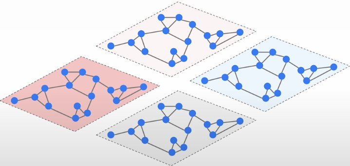
In most vector databases, the HNSW graph is not generated globally; instead, points are separated into non-overlapping segments. Each part will have its own structure constructed. It improves scalability significantly because these segments can be distributed across an entire class of devices. This strategy also increases the system's capacity to function concurrently in a single-node environment while using several CPU cores. It is also much easier to reconstruct this single segment of HNSW graphs because we can do it one at a time. To summarize, changing HNSW settings may provide an additional boost in search quality.
# Tweaking the HNSW Parameters
client.update_collection(
    collection_name="wands-products",
    hnsw_config=models.HnswConfigDiff(
        m=64,
        ef_construct=200,
    )
)
import time

time.sleep(1.0)
collection = client.get_collection("wands-products")
while collection.status != models.CollectionStatus.GREEN:
    time.sleep(1.0)
    collection = client.get_collection("wands-products")

collection
tweaked_run_dict = defaultdict(dict)
for id, row in queries_df.iterrows():
    query_id = f"query_{id}"

    results = client.search(
        collection_name="wands-products",
        query_vector=models.NamedVector(
            name="product_name",
            vector=row["query_embedding"]
        ),
        with_vectors=False,
        with_payload=False,
        limit=100,
        search_params=models.SearchParams(
            exact=False,  # disable exact search
        ),
    )

    for point in results:
        document_id = f"doc_{point.id}"
        tweaked_run_dict[query_id][document_id] = point.score

tweaked_run = Run(
    tweaked_run_dict,
    name="tweaked"
)
tweaked_run
evaluate(
    qrels=qrels,
    run=tweaked_run,
    metrics=["precision@25"]
)
Vector quantization
We will improve an existing vector search technique to reduce memory utilization. You will investigate many methods of vector quantization that not only make semantic search more economical, but also improve its efficiency.
By default, the vectors' dimensions are represented by float32 values. A vector of 1536 dimensions, such as the OpenAI Ada embedding, consumes 6kb of RAM. 1 vector 6kb, 1 million vector 6GB, and 1 billion vector 6TB RAM. There are certain approaches to reduce memory usage by restricting the representation. Quantization approaches proved to be far more powerful, providing a means of making semantic search more economical while having little influence on search quality. The first method you'll learn today is product quantization.
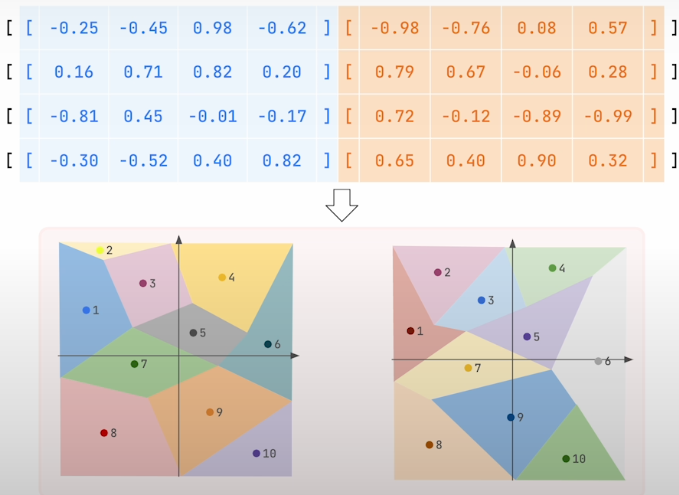
The original vectors are broken into pieces; the larger the number of chunks, the lower the compression rate. The compression rate used determines the number of sub-vectors. For example, a compression rate of 16 indicates that each sub-vector will have four dimensions because the compression rate is measured in bytes. Once the vectors have been separated into pieces, we may begin compression. In the next stage, we begin with sub vectors that will be utilized as input to a clustering method such as k-means. Eventually, each subvector will be assigned to the closest centroid. The number of centroids is not changeable; it is always set at 256. A single byte can encode up to 256 different values. From now on instead of storing the subvectors, we keep the identifiers of the closes centroids. In our case, each subvector had 4 bytes, so it required 16 bytes overall. After the product quantization, we just have to store a single byte which is the centroid identifier.
Sixteen bytes were reduced to a single byte, resulting in an accomplished compression rate of 16. The term "product quantization" refers to the process of dividing a high-dimensional vector into smaller sub-vectors and quantizing each subvector separately using its codebook. The sum of these quantized subvectors is a product of the various code books, resulting in a full product code for the entire space. This method uses the Cartesian product of subspaces to efficiently approximate the original high-dimensional data.
There are several options for product quantization, and the impact varies depending on how you configure it. If you're on a limited budget, you can up the compression rate up to 64 times, but this rarely works well enough.
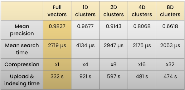
In our situation, the most aggressive compression of 32 times reduced the search precision to approximately 0.66. Even if the search using original vectors yielded approximately 0.98, this is a significant difference. Product quantization will always result in lower search precision, but it may occasionally improve performance. However, inserting your points and constructing the collection will always take longer because the K-means clustering must be conducted. Rescoring can help to enhance the deteriorated quality of quantization.
When searching with quantized vectors, multiple documents may have the same representation. Vector databases often save the original vectors on disk and load them to restore the results. Once we have a collection of quantized search results, we can load the original embeddings and use them to compute similarity. That aids in distinguishing the distances between points in the same neighbourhood. Restoring should improve the quality of search, and turning it off should be a conscious decision.
from qdrant_client import QdrantClient, models

client = QdrantClient("http://localhost:6333", timeout=600)
client.delete_collection("wands-products")
client.recover_snapshot(
    "wands-products",
    "https://storage.googleapis.com/deeplearning-course-c1/snapshots/wands-products.snapshot",
)
collection = client.get_collection("wands-products")
collection

# Test Queries
from sentence_transformers import SentenceTransformer
model = SentenceTransformer("all-MiniLM-L6-v2")

import pandas as pd
queries_df = pd.read_csv(
    "shared_data/WANDS/query.csv",
    sep="\t",
    index_col="query_id",
)
queries_df["query_embedding"] = model.encode(
    queries_df["query"].tolist()
).tolist()
queries_df.sample(n=5)


from collections import defaultdict
from ranx import Qrels

knn_qrels_dict = defaultdict(dict)
for id, row in queries_df.iterrows():
    query_id = f"query_{id}"

    results = client.search(
        collection_name="wands-products",
        query_vector=models.NamedVector(
            name="product_name",
            vector=row["query_embedding"]
        ),
        with_vectors=False,
        with_payload=False,
        limit=50,
        search_params=models.SearchParams(
            exact=True,  # enable exact search
        ),
    )

    for point in results:
        document_id = f"doc_{point.id}"
        # The conversion to integer is required because ranx expects integers
        knn_qrels_dict[query_id][document_id] = int(point.score * 100)

qrels = Qrels(knn_qrels_dict)
qrels

# Product Quantization (PQ)
client.update_collection(
    "wands-products",
    quantization_config=models.ProductQuantization(
        product=models.ProductQuantizationConfig(
            compression=models.CompressionRatio.X64,
            always_ram=True,
        )
    ),
)
import time

time.sleep(1.0)
collection = client.get_collection("wands-products")
while collection.status != models.CollectionStatus.GREEN:
    time.sleep(1.0)
    collection = client.get_collection("wands-products")

collection
import numpy as np

response_times = []
pq_run_dict = defaultdict(dict)
for id, row in queries_df.iterrows():
    query_id = f"query_{id}"

    # Measure the initial time
    start_time = time.monotonic()

    results = client.search(
        collection_name="wands-products",
        query_vector=models.NamedVector(
            name="product_name",
            vector=row["query_embedding"]
        ),
        search_params=models.SearchParams(
            quantization=models.QuantizationSearchParams(
                rescore=False # Disable re-scoring using the original vectors
            )
        ),
        with_vectors=False,
        with_payload=False,
        limit=50,
    )

    # Store the response time in the list
    response_times.append(time.monotonic() - start_time)

    for point in results:
        document_id = f"doc_{point.id}"
        pq_run_dict[query_id][document_id] = point.score

np.mean(response_times)
from ranx import Run, evaluate

product_name_pq_run = Run(
    pq_run_dict,
    name="product_name_pq"
)
evaluate(
    qrels=qrels,
    run=product_name_pq_run,
    metrics=["precision@25"]
)
# 0.826666666666666667
Scalar quantization is another approach you may use to make semantic search less memory heavy. It is based on the extremely simple concept of converting floating to integers. However, when we represent the original vectors with floats, the individual numbers originate from a predefined range, which is only a subset of all the values that can be represented with floats. When we receive fresh vectors, the range can fluctuate, thus we never know the minimum and maximum values.
That is why quantization is performed on subsets of the data rather than on the entire vector set. Because the database assumes that each segment is separable, separating each segment aids Scalar quantization, much as it does with HNSW. So we can determine the range of the integers and calculate the minimum and maximum values. The entire quantization procedure then revolves around converting these numbers from the integer range of 0 to 255, or -128 to 127. Scalar quantization has a constant compression rate of four. Four bytes are compressed into a single one.
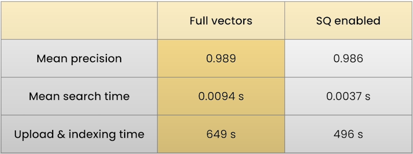
The memory required to retain the vectors after scalar quantization is up to 75% slower. This comes at a cost in terms of search precision, but it also provides speed benefits. Overall, if you want to speed up and lower the cost of your search, scalar quantization is usually the first item to consider.
response_times = []
pq_rescore_run_dict = defaultdict(dict)
for id, row in queries_df.iterrows():
    query_id = f"query_{id}"

    start_time = time.monotonic()

    results = client.search(
        collection_name="wands-products",
        query_vector=models.NamedVector(
            name="product_name",
            vector=row["query_embedding"]
        ),
        search_params=models.SearchParams(
            quantization=models.QuantizationSearchParams(
                rescore=True # Enable re-scoring using the original vectors
            )
        ),
        with_vectors=False,
        with_payload=False,
        limit=50,
    )

    response_times.append(time.monotonic() - start_time)

    for point in results:
        document_id = f"doc_{point.id}"
        pq_rescore_run_dict[query_id][document_id] = point.score

np.mean(response_times)
product_name_pq_rescore_run = Run(
    pq_rescore_run_dict,
    name="product_name_pq_rescore"
)
evaluate(
    qrels=qrels,
    run=product_name_pq_rescore_run,
    metrics=["precision@25"]
)

# Scalar Quantization (SQ)
client.update_collection(
    "wands-products",
    quantization_config=models.ScalarQuantization(
        scalar=models.ScalarQuantizationConfig(
            type=models.ScalarType.INT8,
            always_ram=True,
        )
    ),
)
time.sleep(1.0)
collection = client.get_collection("wands-products")
while collection.status != models.CollectionStatus.GREEN:
    time.sleep(1.0)
    collection = client.get_collection("wands-products")

collection
response_times = []
sq_run_dict = defaultdict(dict)
for id, row in queries_df.iterrows():
    query_id = f"query_{id}"

    start_time = time.monotonic()

    results = client.search(
        collection_name="wands-products",
        query_vector=models.NamedVector(
            name="product_name",
            vector=row["query_embedding"]
        ),
        search_params=models.SearchParams(
            quantization=models.QuantizationSearchParams(
                rescore=False # Disable re-scoring using the original vectors
            )
        ),
        with_vectors=False,
        with_payload=False,
        limit=50,
    )

    response_times.append(time.monotonic() - start_time)

    for point in results:
        document_id = f"doc_{point.id}"
        sq_run_dict[query_id][document_id] = point.score

np.mean(response_times)
product_name_sq_run = Run(
    sq_run_dict,
    name="product_name_sq"
)
evaluate(
    qrels=qrels,
    run=product_name_sq_run,
    metrics=["precision@25"]
)
response_times = []
sq_rescore_run_dict = defaultdict(dict)
for id, row in queries_df.iterrows():
    query_id = f"query_{id}"

    start_time = time.monotonic()

    results = client.search(
        collection_name="wands-products",
        query_vector=models.NamedVector(
            name="product_name",
            vector=row["query_embedding"]
        ),
        search_params=models.SearchParams(
            quantization=models.QuantizationSearchParams(
                rescore=True # Enable re-scoring using the original vectors
            )
        ),
        with_vectors=False,
        with_payload=False,
        limit=50,
    )

    response_times.append(time.monotonic() - start_time)

    for point in results:
        document_id = f"doc_{point.id}"
        sq_rescore_run_dict[query_id][document_id] = point.score

np.mean(response_times)
product_name_sq_rescore_run = Run(
    sq_rescore_run_dict,
    name="product_name_sq_rescore"
)
evaluate(
    qrels=qrels,
    run=product_name_sq_rescore_run,
    metrics=["precision@25"]
)
# 0.99375
Binary quantization shrinks individual dimensions much more. It turns each floating-point number into a boolean value of 0 or 1. 32 bits of information are compressed into a single bit. The role is as simple as changing each positive number to one and each negative value to zero. One key consideration is binary sampling, which represents numerous points in the same way. You want to extract more points than you really require and calculate the distance between your query and the original vectors represented as floats. Let's take a look at the real-world impact of binary quantization.
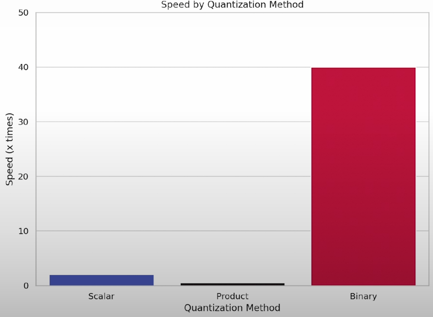
Binary quantization reduces memory use by up to 32 times, but the performance gains could be significantly greater, increasing retrieval speed by up to 40 times. Choosing the appropriate quantization relies on the circumstances of your application.
# Binary Quantization (BQ)
client.update_collection(
    "wands-products",
    quantization_config=models.BinaryQuantization(
        binary=models.BinaryQuantizationConfig(
            always_ram=True,
        )
    ),
)
time.sleep(1.0)
collection = client.get_collection("wands-products")
while collection.status != models.CollectionStatus.GREEN:
    time.sleep(1.0)
    collection = client.get_collection("wands-products")

collection
response_times = []
bq_run_dict = defaultdict(dict)
for id, row in queries_df.iterrows():
    query_id = f"query_{id}"

    start_time = time.monotonic()

    results = client.search(
        collection_name="wands-products",
        query_vector=models.NamedVector(
            name="product_name",
            vector=row["query_embedding"]
        ),
        search_params=models.SearchParams(
            quantization=models.QuantizationSearchParams(
                rescore=False # Disable re-scoring using the original vectors
            )
        ),
        with_vectors=False,
        with_payload=False,
        limit=50,
    )

    response_times.append(time.monotonic() - start_time)

    for point in results:
        document_id = f"doc_{point.id}"
        bq_run_dict[query_id][document_id] = point.score

np.mean(response_times)
product_name_bq_run = Run(
    bq_run_dict,
    name="product_name_bq"
)
evaluate(
    qrels=qrels,
    run=product_name_bq_run,
    metrics=["precision@25"]
)
response_times = []
bq_rescore_run_dict = defaultdict(dict)
for id, row in queries_df.iterrows():
    query_id = f"query_{id}"

    start_time = time.monotonic()

    results = client.search(
        collection_name="wands-products",
        query_vector=models.NamedVector(
            name="product_name",
            vector=row["query_embedding"]
        ),
        search_params=models.SearchParams(
            quantization=models.QuantizationSearchParams(
                rescore=True # Enable re-scoring using the original vectors
            )
        ),
        with_vectors=False,
        with_payload=False,
        limit=50,
    )

    response_times.append(time.monotonic() - start_time)

    for point in results:
        document_id = f"doc_{point.id}"
        bq_rescore_run_dict[query_id][document_id] = point.score

np.mean(response_times)
product_name_bq_rescore_run = Run(
    bq_rescore_run_dict,
    name="product_name_bq_rescore"
)
evaluate(
    qrels=qrels,
    run=product_name_bq_rescore_run,
    metrics=["precision@25"]
)
from ranx import compare

compare(
    qrels=qrels,
    runs=[
        product_name_pq_run,
        product_name_pq_rescore_run,
        product_name_sq_run,
        product_name_sq_rescore_run,
        product_name_bq_run,
        product_name_bq_rescore_run,
    ],
    metrics=["precision@25"],
)
Reference
Deeplearning.ai, (2024), Retrieval Optimization: Tokenization to Vector Quantization:


0 Comments