Introduction
Flower will allow you to create a federated learning system and perform distributed machine learning training jobs in a privacy-friendly manner. Suppose you train a model on x-ray pictures but are unable to collect all of them due to regulations. Federated learning allows you to train on distributed data sources rather than collecting all data centrally. You can move the training to the data rather than the other way around. Run dispersed training jobs across all hospitals after centralizing the model parameters, not the raw data.
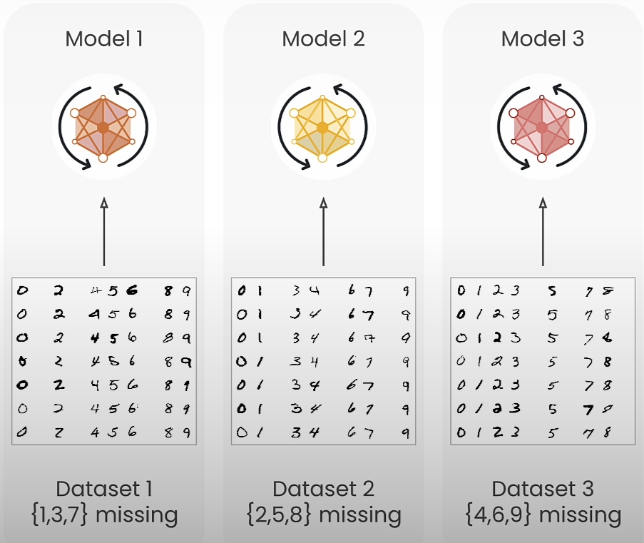
This allows you to create a model that benefits from all of the data collected across all hospitals while never requiring the raw data to leave any of them. In this course, you will investigate this using the MNIST digits dataset, which includes a dataset with some missing digits as well as other datasets with varying missing digits. With federated learning, you train a model using your handwritten digit data while others train on theirs. Then, everyone submits the revised model parameters to the central server, which aggregates updates from all sources to improve the global model without evaluating the individual data sources. This worldwide model is accessible to everybody.
Federated learning enables us to create powerful and accurate models while keeping data within the control of the users and organizations who possess it. By training models locally on various devices or servers, we may use a wide range of data without having to share it centrally. This method is ideal for industries such as healthcare and finance, where data is sensitive and must be protected. Federated learning allows us to train models for tasks that previously lacked adequate or diverse training data.
Let's look at how federated learning works and how it may be tuned. We'll also learn about differential privacy (DP), which is a mechanism for protecting individual data pieces such as messages or photographs. We will receive an overview of the various components and federated learning systems. We will learn how to configure, tune, and orchestrate the many components of federated learning systems.
Why Federated Learning
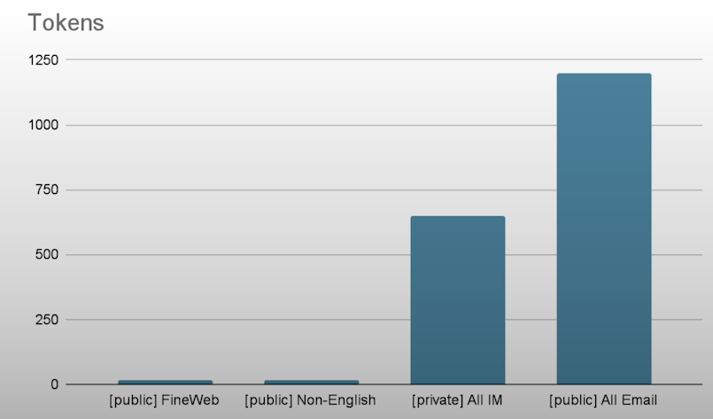
In this course, we'll use Federated Learning to open massive volumes of previously unavailable training data. Llama3 outperforms Llama2 because it was trained with seven times the data and four times the code. There is currently 15 trillion token LLM training data in the globe. LLMs are anticipated to run out of data by 2026. Data, by its very nature, is spread across businesses and consumer devices. Traditional training presupposes centralized data because it only uses a single dataset. The majority of the world's data is not easily accessible for analysis.
from utils1 import *
trainset = datasets.MNIST(
    "./MNIST_data/", download=True, train=True, transform=transform
)
total_length = len(trainset)
split_size = total_length // 3
torch.manual_seed(42)

part1, part2, part3 = random_split(trainset, [split_size] * 3)
part1 = exclude_digits(part1, excluded_digits=[1, 3, 7])
part2 = exclude_digits(part2, excluded_digits=[2, 5, 8])
part3 = exclude_digits(part3, excluded_digits=[4, 6, 9])

plot_distribution(part1, "Part 1")
plot_distribution(part2, "Part 2")
plot_distribution(part3, "Part 3")

model1 = SimpleModel()
train_model(model1, part1)

model2 = SimpleModel()
train_model(model2, part2)

model3 = SimpleModel()
train_model(model3, part3)

testset = datasets.MNIST(
    "./MNIST_data/", download=True, train=False, transform=transform
)

testset_137 = include_digits(testset, included_digits=[1, 3, 7])
testset_258 = include_digits(testset, included_digits=[2, 5, 8])
testset_469 = include_digits(testset, included_digits=[4, 6, 9])

_, accuracy1 = evaluate_model(model1, testset)
_, accuracy1_on_137 = evaluate_model(model1, testset_137)
print(
    f"Model 1-> Test Accuracy on all digits: {accuracy1:.4f}, "
    f"Test Accuracy on [1,3,7]: {accuracy1_on_137:.4f}"
)

_, accuracy2 = evaluate_model(model2, testset)
_, accuracy2_on_258 = evaluate_model(model2, testset_258)
print(
    f"Model 2-> Test Accuracy on all digits: {accuracy2:.4f}, "
    f"Test Accuracy on [2,5,8]: {accuracy2_on_258:.4f}"
)

_, accuracy3 = evaluate_model(model3, testset)
_, accuracy3_on_469 = evaluate_model(model3, testset_469)
print(
    f"Model 3-> Test Accuracy on all digits: {accuracy3:.4f}, "
    f"Test Accuracy on [4,6,9]: {accuracy3_on_469:.4f}"
)

confusion_matrix_model1_all = compute_confusion_matrix(model1, testset)
confusion_matrix_model2_all = compute_confusion_matrix(model2, testset)
confusion_matrix_model3_all = compute_confusion_matrix(model3, testset)

plot_confusion_matrix(confusion_matrix_model1_all, "model 1")
plot_confusion_matrix(confusion_matrix_model2_all, "model 2")
plot_confusion_matrix(confusion_matrix_model3_all, "model 3")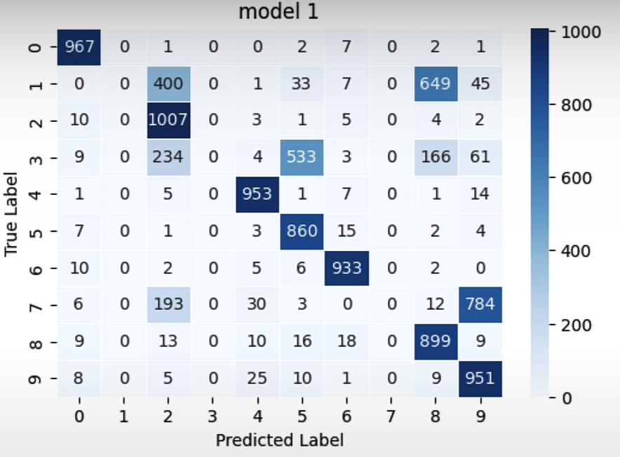
Everyone can keep their data private while yet collaborating with it through federated learning.
In finance, data is strictly regulated. Customers' transactions must stay within the country, although collaboration with other countries is critical for global anti-money laundering frameworks. Another example is user-generated keyboard writing predictions. Another example is when hospitals collaborate on data.
Federated Training Process
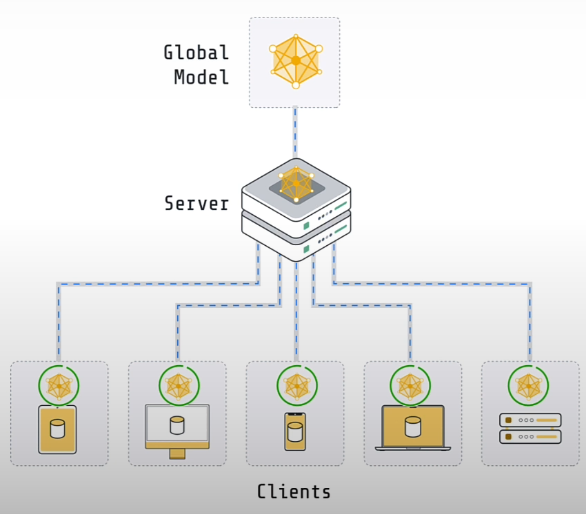
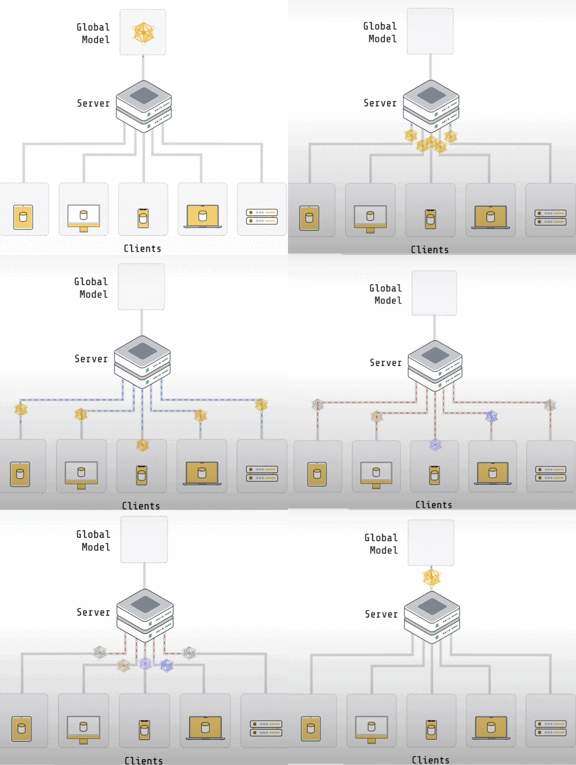
A basic federated learning system consists of a server and clients. Often, there is no data on the server. It may contain some data used to evaluate the global model. However, vanilla federated learning does not include any training data. The clients have the actual training data. If you have a system that allows hospitals to collaborate on model training, you will have five customers, one for each institution. Each of these clients would run in one of the hospital environments and have access to the data specific to that facility.
If you had a system with 100 million user devices storing data, you'd need 100 million clients, one for each user device. The server's role is to coordinate training among multiple clients. The clients' responsibility is to conduct the actual training on their respective local data sets. Both the server and the clients have copies of the model. The model on the server is often referred to as the global model. The models on a client are often referred to as local models.
The entire process begins with the server initializing the global model settings. The server provides the global model's parameters to the client. They only train the model for a short period of time, usually just one epoch on their local data set, before full convergence. Following local training, the client returned their improved models to the server. We now have five models on five clients and want to aggregate them. The most common strategy is to average the weights.
The federated learning algorithm:
- Initialization:
The server initializes the global model.
2. Communication Round:
For each communication round:
- The server sends the global model to participating clients.
- Each client receives the global model.
3. Client Training and Model Update:
For each participating client:
- The client trains the received model on its local dataset.
- The client sends its locally updated model to the server.
4. Model Aggregation:
The server aggregates the updated models received from all clients using an Aggregation algorithm for instance FedAvg.
5. Convergence Check:
If convergence criteria are met, end the FL process if not proceed to the next communication round, the second step.
from flwr.client import Client, ClientApp, NumPyClient
from flwr.common import ndarrays_to_parameters, Context
from flwr.server import ServerApp, ServerConfig
from flwr.server import ServerAppComponents
from flwr.server.strategy import FedAvg
from flwr.simulation import run_simulation

from utils2 import *

trainset = datasets.MNIST(
    "./MNIST_data/", download=True, train=True, transform=transform
)

total_length = len(trainset)
split_size = total_length // 3
torch.manual_seed(42)
part1, part2, part3 = random_split(trainset, [split_size] * 3)

part1 = exclude_digits(part1, excluded_digits=[1, 3, 7])
part2 = exclude_digits(part2, excluded_digits=[2, 5, 8])
part3 = exclude_digits(part3, excluded_digits=[4, 6, 9])

train_sets = [part1, part2, part3]

testset = datasets.MNIST(
    "./MNIST_data/", download=True, train=False, transform=transform
)
print("Number of examples in `testset`:", len(testset))

testset_137 = include_digits(testset, [1, 3, 7])
testset_258 = include_digits(testset, [2, 5, 8])
testset_469 = include_digits(testset, [4, 6, 9])

# Set functions for the client-server exchange of the training information.
# Sets the parameters of the model
def set_weights(net, parameters):
    params_dict = zip(net.state_dict().keys(), parameters)
    state_dict = OrderedDict(
        {k: torch.tensor(v) for k, v in params_dict}
    )
    net.load_state_dict(state_dict, strict=True)

# Retrieves the parameters from the model
def get_weights(net):
    ndarrays = [
        val.cpu().numpy() for _, val in net.state_dict().items()
    ]
    return ndarrays


# Connect the training in the pipeline using the Flower Client.
class FlowerClient(NumPyClient):
    def __init__(self, net, trainset, testset):
        self.net = net
        self.trainset = trainset
        self.testset = testset

    # Train the model
    def fit(self, parameters, config):
        set_weights(self.net, parameters)
        train_model(self.net, self.trainset)
        return get_weights(self.net), len(self.trainset), {}

    # Test the model
    def evaluate(self, parameters: NDArrays, config: Dict[str, Scalar]):
        set_weights(self.net, parameters)
        loss, accuracy = evaluate_model(self.net, self.testset)
        return loss, len(self.testset), {"accuracy": accuracy}

# Flower calls client_fn whenever it needs an instance of one particular client to call fit or evaluate.
# Client function
def client_fn(context: Context) -> Client:
    net = SimpleModel()
    partition_id = int(context.node_config["partition-id"])
    client_train = train_sets[int(partition_id)]
    client_test = testset
    return FlowerClient(net, client_train, client_test).to_client()

client = ClientApp(client_fn)

# The evaluate method evaluates the performance of the neural network model using the provided parameters and the test dataset (testset).
def evaluate(server_round, parameters, config):
    net = SimpleModel()
    set_weights(net, parameters)

    _, accuracy = evaluate_model(net, testset)
    _, accuracy137 = evaluate_model(net, testset_137)
    _, accuracy258 = evaluate_model(net, testset_258)
    _, accuracy469 = evaluate_model(net, testset_469)

    log(INFO, "test accuracy on all digits: %.4f", accuracy)
    log(INFO, "test accuracy on [1,3,7]: %.4f", accuracy137)
    log(INFO, "test accuracy on [2,5,8]: %.4f", accuracy258)
    log(INFO, "test accuracy on [4,6,9]: %.4f", accuracy469)

    if server_round == 3:
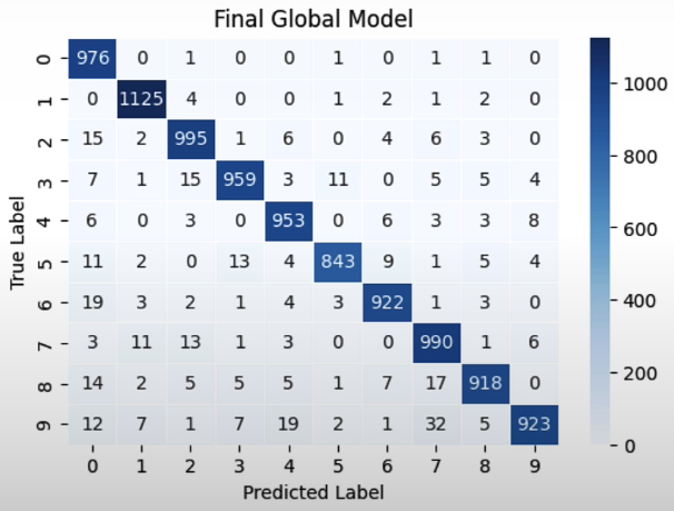
        cm = compute_confusion_matrix(net, testset)
        plot_confusion_matrix(cm, "Final Global Model")

net = SimpleModel()
params = ndarrays_to_parameters(get_weights(net))

def server_fn(context: Context):
    strategy = FedAvg(
        fraction_fit=1.0,
        fraction_evaluate=0.0,
        initial_parameters=params,
        evaluate_fn=evaluate,
    )
    config=ServerConfig(num_rounds=3)
    return ServerAppComponents(
        strategy=strategy,
        config=config,
    )

server = ServerApp(server_fn=server_fn)

# Start training
# Initiate the simulation passing the server and client apps
# Specify the number of super nodes that will be selected on every round
run_simulation(
    server_app=server,
    client_app=client,
    num_supernodes=3,
    backend_config=backend_setup,
)
Tuning
Compared to standard centralized training, federated learning incorporates several new concepts and components into the training process that may be adjusted and tuned. One significant consideration is how you choose the clients who participate in each round. This figure shows five clients. So, rather than providing the global model to all five clients, you may provide a model to only three in the first round. The three clients would proceed as usual. Then, in the next round, you might choose three more clients in a small group environment. Often, the answer is just to select all clients in each round. If you had simply five consumers, as in this diagram, you would most likely select all of them in each round of Federated learning. But then in settings where you have large numbers of clients, you would typically not do this.
It has been demonstrated that selecting more and more clients produces declining profits. Instead, you would select only a subset of available customers in a mobile environment with millions of clients. Depending on the work, you might just select a few hundred clients in a single round, or even a few thousand. There are several ways for picking those clients. A very typical one is to choose them at random. Some ways are not, strictly speaking, federated learning, but they can be quite beneficial. One example is cyclic training, in which the model is sent to one client, trained by that client, returned to the server, and then sent to the next client. And you would do that for one client after another. Another factor is client configuration. Once you’ve selected clients, you need to decide how to configure them. What do you want the client to do?
How long should you train the model? Which hyperparameters should it use? Is there anything more the client should know in order to properly conduct or evaluate the training? The little model symbols on the client are emphasized. This is to identify the client configuration that the client uses to carry out the task. A third example of something that is frequently altered or tuned is aggregation. In federated learning, there are several techniques to aggregating model parameters. You saw and used federated averaging in the last lesson. Many alternative techniques, such as QFedAveraging or FedAdam, offer advantages above traditional federated averaging. Many of them are incorporated into the Flower framework, which you used in the last session, as "strategies."
from flwr.client import Client, ClientApp, NumPyClient
from flwr.server import ServerApp, ServerConfig
from flwr.server.strategy import FedAvg
from flwr.simulation import run_simulation
from flwr_datasets import FederatedDataset

from utils3 import *

def load_data(partition_id):
    fds = FederatedDataset(dataset="mnist", partitioners={"train": 5})
    partition = fds.load_partition(partition_id)

    traintest = partition.train_test_split(test_size=0.2, seed=42)
    traintest = traintest.with_transform(normalize)
    trainset, testset = traintest["train"], traintest["test"]

    trainloader = DataLoader(trainset, batch_size=64, shuffle=True)
    testloader = DataLoader(testset, batch_size=64)
    return trainloader, testloader

def fit_config(server_round: int):
    config_dict = {
        "local_epochs": 2 if server_round < 3 else 5,
    }
    return config_dict

net = SimpleModel()
params = ndarrays_to_parameters(get_weights(net))

def server_fn(context: Context):
    strategy = FedAvg(
        min_fit_clients=5,
        fraction_evaluate=0.0,
        initial_parameters=params,
        on_fit_config_fn=fit_config,  # <- NEW
    )
    config=ServerConfig(num_rounds=3)
    return ServerAppComponents(
        strategy=strategy,
        config=config,
    )

server = ServerApp(server_fn=server_fn)

class FlowerClient(NumPyClient):
    def __init__(self, net, trainloader, testloader):
        self.net = net
        self.trainloader = trainloader
        self.testloader = testloader

    def fit(self, parameters, config):
        set_weights(self.net, parameters)

        epochs = config["local_epochs"]
        log(INFO, f"client trains for {epochs} epochs")
        train_model(self.net, self.trainloader, epochs)

        return get_weights(self.net), len(self.trainloader), {}

    def evaluate(self, parameters, config):
        set_weights(self.net, parameters)
        loss, accuracy = evaluate_model(self.net, self.testloader)
        return loss, len(self.testloader), {"accuracy": accuracy}

def client_fn(context: Context) -> Client:
    net = SimpleModel()
    partition_id = int(context.node_config["partition-id"])
    trainloader, testloader = load_data(partition_id=partition_id)
    return FlowerClient(net, trainloader, testloader).to_client()


client = ClientApp(client_fn)

run_simulation(server_app=server,
               client_app=client,
               num_supernodes=5,
               backend_config=backend_setup
               )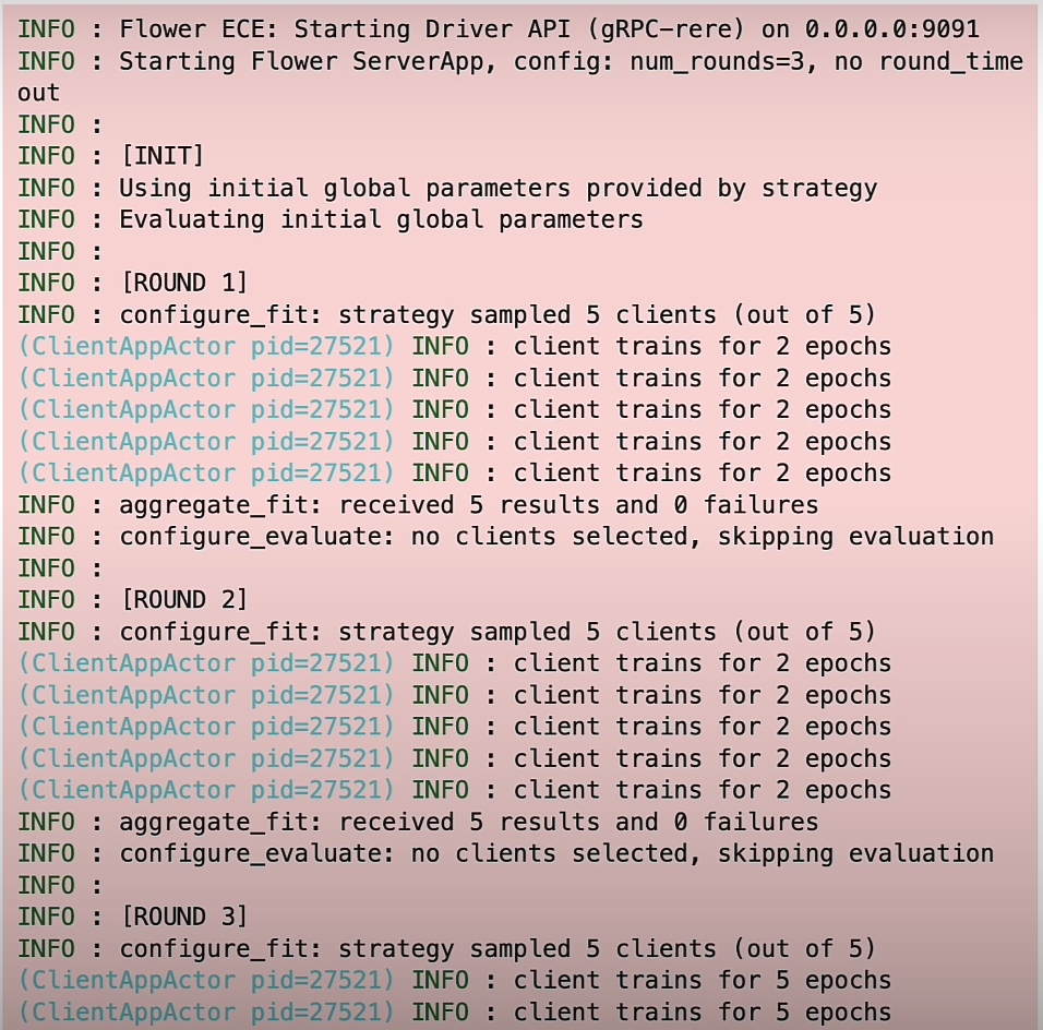
The Flower server app begins and completes three rounds of federated learning. It sets up the strategy's global settings before moving on to the first round.
Data Privacy
Federated learning is a data minimization approach that prohibits direct access to data. However, the model update communication between client and server may still result in privacy leakage. The enemy can be the client, the server, or a third-party.
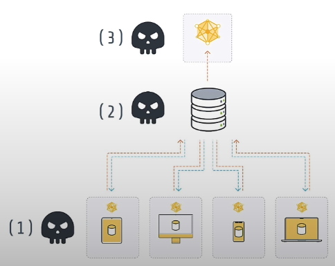
There are three types of privacy attacks: membership inference attacks, which try to infer the participation of data samples, attribute inference attacks, which infer previously unseen features of the training data, and reconstruction attacks, which infer specific training data samples.
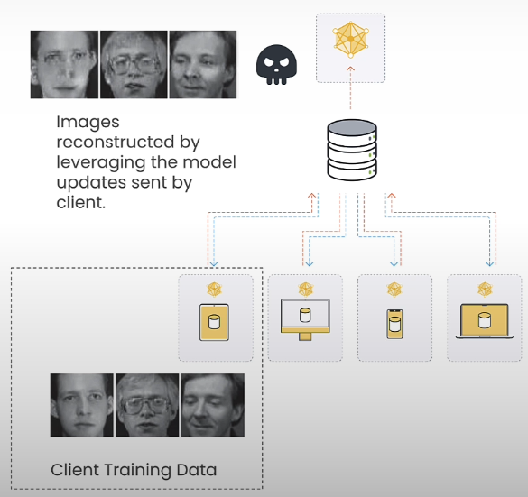
As you can see, photos with surprisingly near source data can be rebuilt.
Differential privacy is a popular solution for improving privacy during data processing. It obscures individual data by introducing calibrated noise into query results, ensuring that the presence or absence of a single data point has no major impact on the analysis's outcome. This provides reliable analysis while protecting sensitive information.
There are two types of differential privacy: central DP and local DP. There are two significant themes in DP: clipping, which limits the sensitivity and reduces the influence of outliers, and noising, which adds calibrated noise to make the result statistically indistinguishable. Sensitivity refers to the maximum amount that the output can change when a single data point is added or withdrawn from the dataset.
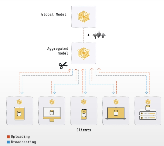
In central differential privacy, the central server adds noise to the globally aggregated parameters. It is important to note that the server must be trusted. The overall strategy is to trim the model updates given by the clients and then add some noise to the aggregated model.
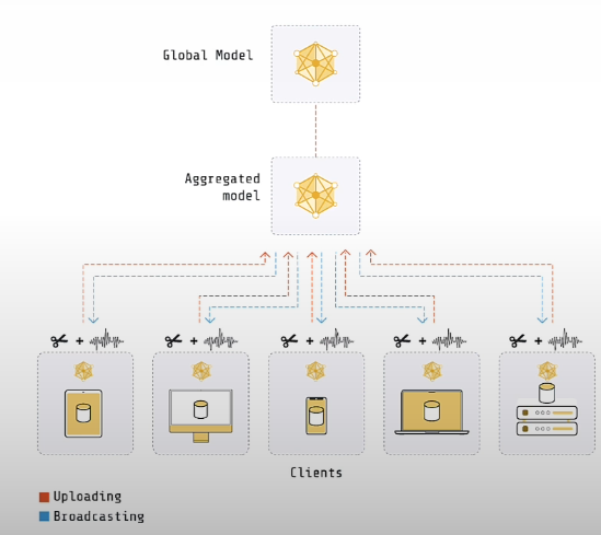
Differential Privacy is performed by each client in a local setting. Local DP eliminates the need for a completely trusted aggregator. Each client is responsible for conducting clipping and noise reduction locally before sending the revised model to the server.
from flwr.client.mod import adaptiveclipping_mod
from flwr.server.strategy import (
    DifferentialPrivacyClientSideAdaptiveClipping,
    FedAvg,
)

from utils4 import *

def load_data(partition_id):
    fds = FederatedDataset(dataset="mnist", partitioners={"train": 10})
    partition = fds.load_partition(partition_id)

    traintest = partition.train_test_split(test_size=0.2, seed=42)
    traintest = traintest.with_transform(normalize)
    trainset, testset = traintest["train"], traintest["test"]

    trainloader = DataLoader(trainset, batch_size=64, shuffle=True)
    testloader = DataLoader(testset, batch_size=64)
    return trainloader, testloader

class FlowerClient(NumPyClient):
    def __init__(self, net, trainloader, testloader):
        self.net = net
        self.trainloader = trainloader
        self.testloader = testloader

    def fit(self, parameters, config):
        set_weights(self.net, parameters)
        train_model(self.net, self.trainloader)
        return get_weights(self.net), len(self.trainloader), {}

    def evaluate(self, parameters, config):
        set_weights(self.net, parameters)
        loss, accuracy = evaluate_model(self.net, self.testloader)
        return loss, len(self.testloader), {"accuracy": accuracy}


def client_fn(context: Context) -> Client:
    net = SimpleModel()
    partition_id = int(context.node_config["partition-id"])
    trainloader, testloader = load_data(partition_id=partition_id)
    return FlowerClient(net, trainloader, testloader).to_client()

client = ClientApp(
    client_fn,
    mods=[adaptiveclipping_mod],  # modifiers
)

net = SimpleModel()
params = ndarrays_to_parameters(get_weights(net))

def server_fn(context: Context):
    fedavg_without_dp = FedAvg(
        fraction_fit=0.6,
        fraction_evaluate=1.0,
        initial_parameters=params,
    )
    fedavg_with_dp = DifferentialPrivacyClientSideAdaptiveClipping(
        fedavg_without_dp,  # <- wrap the FedAvg strategy
        noise_multiplier=0.3,
        num_sampled_clients=6,
    )

    # Adjust to 50 rounds to ensure DP guarantees hold
    # with respect to the desired privacy budget
    config = ServerConfig(num_rounds=5)

    return ServerAppComponents(
        strategy=fedavg_with_dp,
        config=config,
    )

server = ServerApp(server_fn=server_fn)

run_simulation(server_app=server,
               client_app=client,
               num_supernodes=10,
               backend_config=backend_setup
               )
Bandwidth
Let's learn how to reason about federated system bandwidth usage in principle, as well as how to monitor bandwidth consumption in practice with Flower.
As LLMs become larger in generative AI, it is critical to understand the bandwidth consequences.
This formula can be used to estimate the bandwidth required to run a federated learning system:
(model size out + model size in) * cohort size * fraction selected * number of rounds
Sometimes the model size in and out is not equal since we communicate complete model parameters and the client returns compressed gradients. As a result, the update we receive from the client is lower in size than the model we sent out.
Example calculation:
Eluther's Pythia 14M model has a size of 53 MB. We'll transmit the model and get it back from the client. We will train this model with two clients. Because we have two clients, we will select both of them in a single round, so the fraction selected is one (if the cohort size was 100, selecting 50 of them would be a better approach, so the fraction selected would be 0.5). We'll do one round of federated learning. So, the final calculation:
53 MB * 2 * 2 * 1.0 * 1 = 212 MB
We can assess bandwidth using client-side modes, Flower, and server-side techniques to determine server-side and client-side bandwidth needs.
To reduce bandwidth utilization, you can reduce update size by sparsification and quantization, or communicate less by using pre-trained models and training for more epochs.
from flwr.client.mod import parameters_size_mod
from utils5 import *

model = AutoModelForCausalLM.from_pretrained(
    "EleutherAI/pythia-14m",
    cache_dir="./pythia-14m/cache",
)

vals = model.state_dict().values()
total_size_bytes = sum(p.element_size() * p.numel() for p in vals)
total_size_mb = int(total_size_bytes / (1024**2))
log(INFO, "Model size is: {} MB".format(total_size_mb))

class FlowerClient(NumPyClient):
    def __init__(self, net):
        self.net = net

    def fit(self, parameters, config):
        set_weights(self.net, parameters)
        # No actual training here
        return get_weights(self.net), 1, {}

    def evaluate(self, parameters, config):
        set_weights(self.net, parameters)
        # No actual evaluation here
        return float(0), int(1), {"accuracy": 0}


def client_fn(context: Context) -> FlowerClient:
    return FlowerClient(model).to_client()


client = ClientApp(
    client_fn,
    mods=[parameters_size_mod],
)

# Custom Strategy BadnwidthTrackingFedAvg
bandwidth_sizes = []


class BandwidthTrackingFedAvg(FedAvg):
    def aggregate_fit(self, server_round, results, failures):
        if not results:
            return None, {}

        # Track sizes of models received
        for _, res in results:
            ndas = parameters_to_ndarrays(res.parameters)
            size = int(sum(n.nbytes for n in ndas) / (1024**2))
            log(INFO, f"Server receiving model size: {size} MB")
            bandwidth_sizes.append(size)

        # Call FedAvg for actual aggregation
        return super().aggregate_fit(server_round, results, failures)

    def configure_fit(self, server_round, parameters, client_manager):
        # Call FedAvg for actual configuration
        instructions = super().configure_fit(
            server_round, parameters, client_manager
        )

        # Track sizes of models to be sent
        for _, ins in instructions:
            ndas = parameters_to_ndarrays(ins.parameters)
            size = int(sum(n.nbytes for n in ndas) / (1024**2))
            log(INFO, f"Server sending model size: {size} MB")
            bandwidth_sizes.append(size)

        return instructions

params = ndarrays_to_parameters(get_weights(model))

def server_fn(context: Context):
    strategy = BandwidthTrackingFedAvg(
        fraction_evaluate=0.0,
        initial_parameters=params,
    )
    config = ServerConfig(num_rounds=1)
    return ServerAppComponents(
        strategy=strategy,
        config=config,
    )


server = ServerApp(server_fn=server_fn)

run_simulation(server_app=server,
               client_app=client,
               num_supernodes=2,
               backend_config=backend_setup
               )

log(INFO, "Total bandwidth used: {} MB".format(sum(bandwidth_sizes)))
Resource
[https://learn.deeplearning.ai/courses/intro-to-federated-learning/]

0 Comments