Learning Model Quantization in Depth

Introduction

You will learn how to quantize large language models. You will implement the most frequent forms of linear quantization known as asymmetric and symmetric modes, which refer to whether the compression method maps zero in the original representation to zero in the decompress representation, or if it is permitted to move the location of that zero. You will also use PyTorch to create other types of quantization, such as per tensor, per channel, and group quantization, allowing you to specify how large a portion of your model to quantize at once. You create a quantizer that can quantize any model with 8-bit precision by using per-channel linear quantization. Don't be concerned if some of the phrases I use are unfamiliar to you.

Overview

Quantization strategies are used to reduce model size, making them more accessible to the AI community. Let's first define quantization and explain how it works.

Quantization stores the model's parameters with reduced precision. Knowledge distillation allows you to train a smaller student model using the original larger teacher model (which will not be discussed in this session). Pruning removes weighted connections from the model (not covered in this course).

We also discussed common machine learning datatypes like INT8 and float. We'll also employ linear quantization with Huggingface's quantum library, which requires only a few lines of code. Finally, we discussed the applications of quantization.

After watching this course, you will be able to create your own 8-bit linear quantizer and apply it to real-world models. If the model is linear, you can use your linear quantizer to any model, including text, speech, and vision models.

PyTorch does not support two- or four-bit precision weights. One solution to this problem is to compress low-precision weights into higher-precision tensors, such as INT8. We shall learn these using packing and unpacking algorithms.

Quantize and Dequantize a Tensor

Let's build the asymmetric variation of linear quantization from scratch and learn about the scaling factor and zero point.

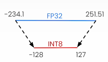
The process of mapping a large set to a smaller set of values is known as quantization. There are other quantisation methods available, however we will only cover linear quantization in this course.

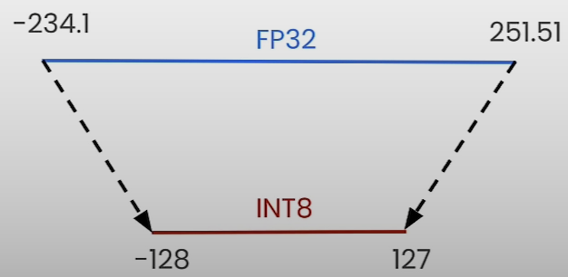
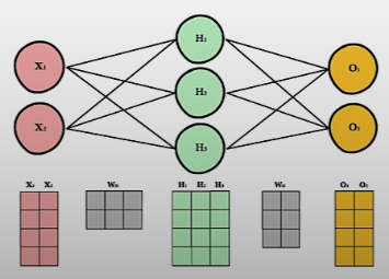
On the left, you can see the 8-bit quantization and map values from torch.float32 to torch.int8 (e.g., [-128, 127]).

We'll learn how to get both the quantized and original tensors.

Weights (neural network parameters) and activations (values that propagate through the neural network's layers) can both be quantified in neural network quantization. If you quantize the NN after it has been trained, you are performing post-training quantification (PTQ).

The benefits of quantization include a smaller model, reduced memory bandwidth, and lower latency as operations (such as GEMM: General Matrix Multiplication and GEMV: Matrix to Vector Multiplication) can be performed more quickly.

Quantization presents numerous issues, including quantization error, retraining (quantization-aware training), restricted hardware support, the necessity for a calibration dataset, and packing/unpacking.

8-bit linear quantization example

r = s (q — z) where s stands for scale and z stands for zero point

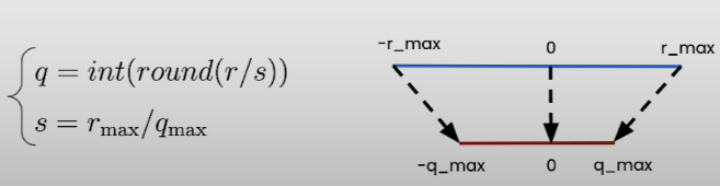
To get the quantized tensor you need to isolate q.

q = int(round(r/s + z))

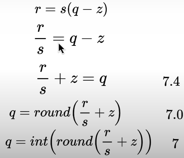
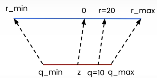
Let us now go on to linear quantization theory. Linear quantization employs linear mapping to convert a higher precision range, such as floating point 32, to an integer. There are two parameters in linear quantization.

Let us take a brief example:

For s=2 and z=0 we get r= 2(q — 0) = 2q. For q=10, we have r= 2*10=20

Quantization with Random Scale and Zero Point

import torch

def linear_q_with_scale_and_zero_point(tensor, scale, zero_point, dtype = torch.int8):
    scaled_and_shifted_tensor = tensor / scale + zero_point
    rounded_tensor = torch.round(scaled_and_shifted_tensor)
    q_min = torch.iinfo(dtype).min
    q_max = torch.iinfo(dtype).max
    q_tensor = rounded_tensor.clamp(q_min,q_max).to(dtype)
    return q_tensor
### a dummy tensor to test the implementation
test_tensor=torch.tensor(
    [[191.6, -13.5, 728.6],
     [92.14, 295.5,  -184],
     [0,     684.6, 245.5]]
)
### these are random values for "scale" and "zero_point"
### to test the implementation
scale = 3.5
zero_point = -70
quantized_tensor = linear_q_with_scale_and_zero_point(
    test_tensor, scale, zero_point)
print(quantized_tensor)

Dequantization with Random Scale and Zero Point

dequantized_tensor = scale * (quantized_tensor.float() - zero_point)
# this was the original tensor
# [[191.6, -13.5, 728.6],
#  [92.14, 295.5,  -184],
#  [0,     684.6, 245.5]]
print(dequantized_tensor)
### without casting to float
scale * (quantized_tensor - zero_point)
def linear_dequantization(quantized_tensor, scale, zero_point):
    return scale * (quantized_tensor.float() - zero_point)
dequantized_tensor = linear_dequantization(quantized_tensor, scale, zero_point)
print(dequantized_tensor)

Quantization Error

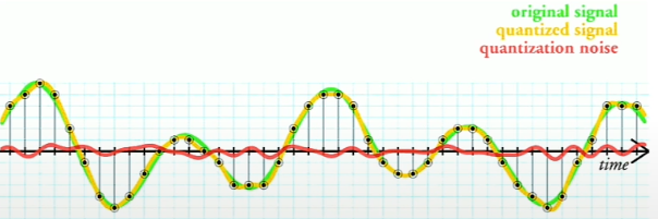
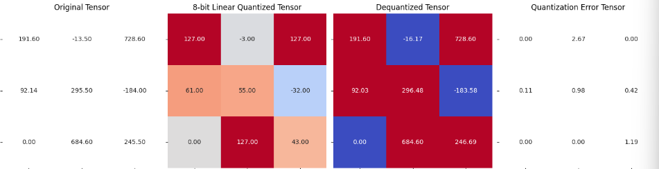
Using the Mean Squared Error approach, determine the "overall" quantization error.

from helper import plot_quantization_errors
plot_quantization_errors(test_tensor, quantized_tensor, dequantized_tensor)
dequantized_tensor - test_tensor
(dequantized_tensor - test_tensor).square()
(dequantized_tensor - test_tensor).square().mean()

Get the Scale and Zero Point

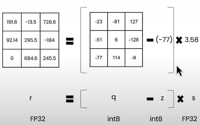
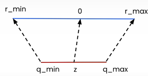
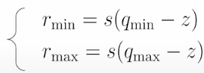
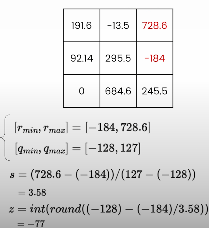
How to determine s (scale) and z (zero point) in r = s*(q-z) equation. Linear quantization maps the floating point range [r_min, r_max] to the quantized range [q_min, q_max].

If we look at the extreme values, we should get:

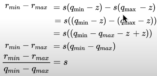
If we subtract the first equation from the second one, we get the scale s:

s = (r_max -r_min) / (q_max — q_min)

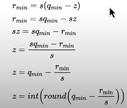
For the zero point z, we need to round the value since it is a n-bit integer:

z = int(round(q_min -r_min/s))

(optional) Scale derivation

(optional) Zero point derivation

Represent zero (in the original "r" range) as an integer in the quantized "q" range. Zero-padding in convolutional neural networks, for example, makes use of tensors that are exactly zero.

Let us use an example to demonstrate how we determine the scale and zero point:

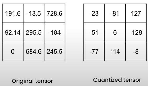
First, we must determine the maximum and minimum ranges of the original tensor. We set the minimum value to -184 and the highest value to 728.6. Because we're quantizing in INT8, the least is -128 and the highest is 127. The r = s*(q- z) formula yields a result.

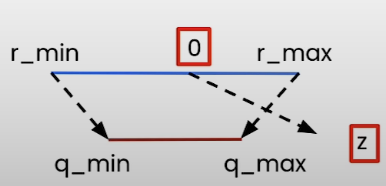
When zero point is out of range:

• Case 1 (z < q_min): We set z= q_min

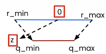
• Case 2 (z > q_max): We set z = q_max

import torch
from helper import linear_q_with_scale_and_zero_point, linear_dequantization, plot_quantization_errors
### a dummy tensor to test the implementation
test_tensor=torch.tensor(
    [[191.6, -13.5, 728.6],
     [92.14, 295.5,  -184],
     [0,     684.6, 245.5]]
)
# Finding scale and zero point for quantization
q_min = torch.iinfo(torch.int8).min
q_max = torch.iinfo(torch.int8).max
print(q_min) # -128
print(q_max) # 127
r_min = test_tensor.min().item()
r_max = test_tensor.max().item()
print(r_min) # -184.0
print(r_max) # 728.5999755859375
scale = (r_max - r_min) / (q_max - q_min)
zero_point = q_min - (r_min / scale)
print(scale) # 3.578893433670343
print(zero_point) # -76.58645490333825
zero_point = int(round(zero_point))
print(zero_point) # - 77

If you put all of this in a function:

def get_q_scale_and_zero_point(tensor, dtype=torch.int8):
    q_min, q_max = torch.iinfo(dtype).min, torch.iinfo(dtype).max
    r_min, r_max = tensor.min().item(), tensor.max().item()
    scale = (r_max - r_min) / (q_max - q_min)
    zero_point = q_min - (r_min / scale)
    # clip the zero_point to fall in [quantized_min, quantized_max]
    if zero_point < q_min:
        zero_point = q_min
    elif zero_point > q_max:
        zero_point = q_max
    else:
        # round and cast to int
        zero_point = int(round(zero_point))
    
    return scale, zero_point

Now test the implementation using the test_tensor we defined at the beginning:

new_scale, new_zero_point = get_q_scale_and_zero_point(test_tensor)
print(new_scale) # 3.578823433670343
print(new_zero_point) # -77

Quantization and dequantization with calculated scale and zero point

Use the calculated scale and zero_point with the functions linear_q_with_scale_and_zero_point and linear_dequantization.

quantized_tensor = linear_q_with_scale_and_zero_point(
    test_tensor, new_scale, new_zero_point)
dequantized_tensor = linear_dequantization(quantized_tensor,
                                           new_scale, new_zero_point)

Plot to see how the quantization error looks like after using calculated scale and zero_point:

plot_quantization_errors(test_tensor, quantized_tensor, 
                         dequantized_tensor)
(dequantized_tensor-test_tensor).square().mean() # tensor(1.5730)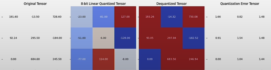

Putting all together: Your linear quantizer:

def linear_quantization(tensor, dtype=torch.int8):
    scale, zero_point = get_q_scale_and_zero_point(tensor, 
                                                   dtype=dtype)
    quantized_tensor = linear_q_with_scale_and_zero_point(tensor,
                                                          scale, 
                                                          zero_point, 
                                                          dtype=dtype)
    return quantized_tensor, scale , zero_point

# Testing your implementation on a random matrix
r_tensor = torch.randn((4, 4))
print(r_tensor)
"""
tensor([[ 0.6859,  1.2172,  0.0154, -1.3982],
        [-0.5769, -0.8755, -1.6292,  3.1698],
        [-1.2492,  0.9837, -0.5668,  1.0646],
        [ 2.3798, -1.2179,  0.6119, -0.9990]])
"""
quantized_tensor, scale, zero_point = linear_quantization(r_tensor)
print(quantized_tensor)
"""
tensor([[ -5, 24, -40, -115],
        [-72, -88, -128, 127],
        [-107, 11, -71, 16],
        [ 85, -106, -8, -94]], dtype=torch.int8)
"""
print(scale) # 0.018819578021180398
print(zero_point) # -41
dequantized_tensor = linear_dequantization(quantized_tensor,
                                           scale, zero_point)
plot_quantization_errors(r_tensor, quantized_tensor,
                         dequantized_tensor)
(dequantized_tensor-r_tensor).square().mean()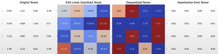

Symmetric vs Asymmetric Mode

You will learn about symmetric and asymmetric modes and how to implement quantization at various granularities, including per tensor, per channel, and per group quantization. Finally, you will learn how to infer on the quantized linear layer.

There are 2 modes of linear quantization:

• Symmetric: We map [-rmax, rmax] to [-qmax, qmax] where we can set rmax = max(|r_tensor|).

We do not have to use the zero point (z=0). This occurs because the floating-point and quantized ranges are symmetric around zero. Therefore, we can simplify the equation to:

• Asymmetric: We map [rmin, rmax] to [qmin, qmax]. This is what we implemented in the previous chapter.

Symmetric Linear Quantization

import torch
# Returns the scale for Linear Quantization in Symmetric Mode.
def get_q_scale_symmetric(tensor, dtype=torch.int8):
    r_max = tensor.abs().max().item()
    q_max = torch.iinfo(dtype).max
    # return the scale
    return r_max/q_max

### test the implementation on a 4x4 matrix
test_tensor = torch.randn((4, 4))
get_q_scale_symmetric(test_tensor) # 0.01664387710451141

Performing Linear Quantization in Symmetric Mode. linear_q_with_scale_and_zero_point is the same function you implemented in the previous lesson.

from helper import linear_q_with_scale_and_zero_point
def linear_q_symmetric(tensor, dtype=torch.int8):
    scale = get_q_scale_symmetric(tensor)
    quantized_tensor = linear_q_with_scale_and_zero_point(tensor,
                                                     scale=scale,
                                                    zero_point=0, # in symmetric quantization zero point is = 0
                                                      dtype=dtype)
    return quantized_tensor, scale

quantized_tensor, scale = linear_q_symmetric(test_tensor)

Dequantization

Perform quantization and plot the quantization error; linear_dequantization is the same function you used in the last lesson.

from helper import linear_dequantization, plot_quantization_errors
from helper import quantization_error
dequantized_tensor = linear_dequantization(quantized_tensor,scale,0)
plot_quantization_errors(test_tensor, quantized_tensor, dequantized_tensor)

print(f"""Quantization Error : {quantization_error(test_tensor, dequantized_tensor)}""") # Quanztization Error: 2.5686615117592737e-05

Trade-off:

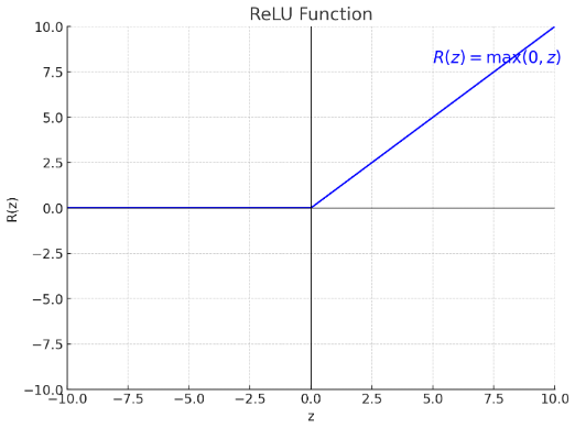
• Quantized range utilization: Asymmetric quantization completely utilizes the quantized range. If the float range is skewed to one side in symmetric mode, a quantized range will result, with a portion of the range allocated to values that will never be seen.(For example, ReLU yields positive results).
  * Simplicity: Symmetric mode is much simpler than asymmetric mode.
  * Memory: For symmetric quantization, we do not store the zero point.
  

Finer Granularity for more Precision

The coloured values share the same quantization parameters (e.g. scale, zero point).

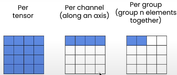
The finer the quantization, the more precise it will be. However, it consumes more memory because we need to store more quantization settings. There are several levels of granularity when it comes to quantification. We have per-tensor quantization, but as you can see, we do not need to utilize the same scale and zero point for the entire tensor. For example, we can calculate a scale and zero point for each axis. This is known as per-channel quantization. We might also select a group of n components to obtain the scale and zero points, and then quantify each group using the scale and zero points.

import torch

from helper import linear_q_symmetric, get_q_scale_symmetric, linear_dequantization
from helper import plot_quantization_errors, quantization_error

Let’s perform different granularities for quantization but for simplicity use symmetric mode.

Per Tensor Symmetric Quantization

# test tensor
test_tensor=torch.tensor(
    [[191.6, -13.5, 728.6],
     [92.14, 295.5,  -184],
     [0,     684.6, 245.5]]
)
quantized_tensor, scale = linear_q_symmetric(test_tensor)
dequantized_tensor = linear_dequantization(quantized_tensor, scale, 0)
plot_quantization_errors(test_tensor, quantized_tensor, dequantized_tensor)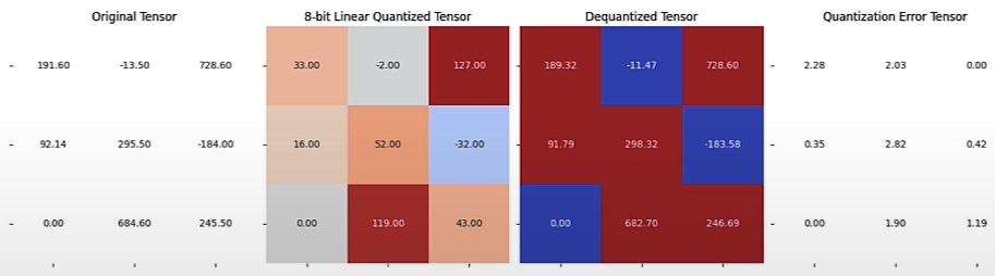

print(f"""Quantization Error : {quantization_error(test_tensor, dequantized_tensor)}""")
# Quantization Error: 2.5091912746429443

Per Channel Quantization

Per channel quantization along an axis. The coloured values share the same quantization parameters (e.g scale, zero point)

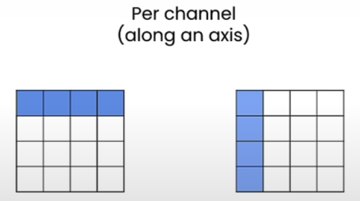
If we prefer to quantize along the rows, we must store the scales and zero point for each row, and if we choose to quantize along the columns, we must store them along each column. The memory required to hold all of these linear parameters is rather little. When it comes to eight-bit models, we typically utilize per-channel quantization. You will see that we employ units in the next lesson.

Let us implement per-channel symmetric quantization. The dim option determines whether it should be along the rows and columns.

import torch
from helper import get_q_scale_symmetric, linear_q_with_scale_and_zero_point, linear_dequantization
from helper import plot_quantization_errors, quantization_error

def linear_q_symmetric_per_channel(tensor,dim,dtype=torch.int8):
    return quantized_tensor, scale
test_tensor=torch.tensor(
    [[191.6, -13.5, 728.6],
     [92.14, 295.5,  -184],
     [0,     684.6, 245.5]]
)
dim=0
output_dim = test_tensor.shape[dim]
print(output_dim)
scale = torch.zeros(output_dim)
print(scale) # tensor([5.7370, 2.3268, 5.3906])
scale_shape = [1] * test_tensor.dim()
print(scale_shape) # [1, 1]
scale_shape[dim] = -1
print(scale_shape) # [1, 1]
scale = scale.view(scale_shape)
copy_scale = scale # copied to be used later
m = torch.tensor([[1,2,3],[4,5,6],[7,8,9]])
print(m) # tensor([[1,2,3], [4,5,6], [7,8,9]])
s = torch.tensor([1,5,10])
print(s) # tensor([1, 5, 10])
print(s.shape) # torch.Size([3])
s.view(1, 3).shape
s.view(1, -1).shape # alternate way
s.view(-1,1).shape
scale = torch.tensor([[1], [5], [10]])
print(scale.shape) # torch.Size([3, 1])
print(m / scale) # tensor([[1.0000,2.0000,3.0000], [0.8000,1.0000,1.2000], [0.7000,0.8000,0.9000]])
scale = torch.tensor([[1, 5, 10]])
print(scale.shape) # torch.Size([1, 3])
print(m / scale) # tensor([[1.0000,0.4000,0.3000], [4.0000,1.0000,0.6000], [7.0000,1.6000,0.9000]])
# the scale you got earlier
scale = copy_scale
print(scale) # tensor([[5.7370],[2.3268],[5.3906]])
print(scale.shape) # torch.Size([3,1])
quantized_tensor = linear_q_with_scale_and_zero_point( test_tensor, scale=scale, zero_point=0)
print(quantized_tensor) # tensor([[33, -2 , 127],[40, 127, -79],[0, 127, 46]])
def linear_q_symmetric_per_channel(r_tensor, dim, dtype=torch.int8):
    output_dim = r_tensor.shape[dim]
    # store the scales
    scale = torch.zeros(output_dim)
    for index in range(output_dim):
        sub_tensor = r_tensor.select(dim, index)
        scale[index] = get_q_scale_symmetric(sub_tensor, dtype=dtype)
    # reshape the scale
    scale_shape = [1] * r_tensor.dim()
    scale_shape[dim] = -1
    scale = scale.view(scale_shape)
    quantized_tensor = linear_q_with_scale_and_zero_point(
        r_tensor, scale=scale, zero_point=0, dtype=dtype)
    return quantized_tensor, scale

test_tensor=torch.tensor(
    [[191.6, -13.5, 728.6],
     [92.14, 295.5,  -184],
     [0,     684.6, 245.5]]
)
### along the rows (dim = 0)
quantized_tensor_0, scale_0 = linear_q_symmetric_per_channel(
    test_tensor, dim=0)
### along the columns (dim = 1)
quantized_tensor_1, scale_1 = linear_q_symmetric_per_channel(
    test_tensor, dim=1)
# Plot the quantization error for along the rows
dequantized_tensor_0 = linear_dequantization(quantized_tensor_0, scale_0, 0)
plot_quantization_errors(test_tensor, quantized_tensor_0, dequantized_tensor_0)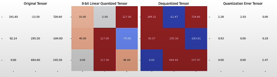

print(f"""Quantization Error : {quantization_error(test_tensor, dequantized_tensor_0)}""")
# Quantization Error: 1.8084441423416138

dequantized_tensor_1 = linear_dequantization(quantized_tensor_1, scale_1, 0)
plot_quantization_errors(test_tensor, quantized_tensor_1, dequantized_tensor_1, n_bits=8)

print(f"""Quantization Error : {quantization_error(test_tensor, dequantized_tensor_1)}""")
# Quantization Error: 1.0781488418579102

Hallucinations continue to be a significant issue for big language models. Models are prone to overconfidence, even in fields in which they have little understanding. Despite these flaws, they are frequently utilized as knowledge bases, which can result in undesirable results such as the propagation of disinformation. While we acknowledge that factuality can extend beyond hallucinations, we focused on hallucinations here.

Per Group Quantization

Per-group quantization can demand significantly more memory. Assume we wish to quantize a tensor in 4-bits and use group_size=32, symmetric mode(z=0), and store the scales in FP16. It means that we quantize the tensor in 4.5 bits, because we have:

• 4-bit (each element is stored in 4-bit)
• 16/32 bit (scale in 16 bits for every 32 elements)

Let us put our plans into action. For the sake of simplicity, we shall limit ourselves to employing the symmetric mode with a two-dimensional tensor.

import torch
from helper import linear_q_symmetric_per_channel, get_q_scale_symmetric, linear_dequantization
from helper import plot_quantization_errors, quantization_error

For simplicity, you’ll quantize a 2D tensor along the rows.

def linear_q_symmetric_per_group(tensor, group_size, dtype=torch.int8):
    t_shape = tensor.shape # to get rows of group size elements
    assert t_shape[1] % group_size == 0
    assert tensor.dim() == 2
    tensor = tensor.view(-1, group_size)
    quantized_tensor, scale = linear_q_symmetric_per_channel(tensor, dim=0, dtype=dtype)
    quantized_tensor = quantized_tensor.view(t_shape)
    return quantized_tensor, scale

def linear_dequantization_per_group(quantized_tensor, scale, group_size):
    q_shape = quantized_tensor.shape
    quantized_tensor = quantized_tensor.view(-1, group_size)
    dequantized_tensor = linear_dequantization(quantized_tensor, scale, 0)
    dequantized_tensor = dequantized_tensor.view(q_shape)
    return dequantized_tensor
test_tensor = torch.rand((6, 6))
group_size = 3
quantized_tensor, scale = linear_q_symmetric_per_group(test_tensor, group_size=group_size)
dequantized_tensor = linear_dequantization_per_group(quantized_tensor, scale, group_size=group_size)
plot_quantization_errors(test_tensor, quantized_tensor, dequantized_tensor)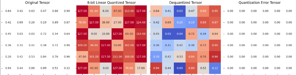

print(f"""Quantization Error : {quantization_error(test_tensor, dequantized_tensor)}""")
# Quantization Error: 2.150184179332227e^-06

Quantizing Weights & Activations for Inference

In a neural network, we can measure both the weights and the activation. Depending on what we measure, storage and computation are not the same.

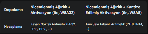
It is important to note that we must dequantize the weights to execute floating point computations in floating point arithmetics since integer-based arithmetic is not supported by all hardware.

W8A32 represents 8-bit weights and 32-bit activations. For simplicity, the linear layer will be bias-free.

import torch
from helper import linear_q_symmetric, get_q_scale_symmetric

def quantized_linear_W8A32_without_bias(input, q_w, s_w, z_w):
    assert input.dtype == torch.float32
    assert q_w.dtype == torch.int8
    dequantized_weight = q_w.to(torch.float32) * s_w + z_w
    output = torch.nn.functional.linear(input, dequantized_weight)
    return output
input = torch.tensor([1, 2, 3], dtype=torch.float32)
weight = torch.tensor([[-2,   -1.13, 0.42],
                       [-1.51, 0.25, 1.62],
                       [0.23,  1.35, 2.15]])
q_w, s_w  = linear_q_symmetric(weight)
print(q_w) # tensor([[-118, -67, 25],[-89, 15, 96],[14, 80, 127]], dtype=torch.int8)
print(s_w) # 0.016929134609192376
output = quantized_linear_W8A32_without_bias(input, q_w, s_w, 0)
print(f"This is the W8A32 output: {output}")
# This is the W8A32 output: tensor([-2.9965, 3.8768, 9.3957])
fp32_output = torch.nn.functional.linear(input, weight)
print(f"This is the output if we don't quantize: {fp32_output}")
# This is the output if we don't quantize: tensor([-3.000, 3.8500, 9.3800])

Custom Build an 8-bit Quantizer

We will learn to create a W8A16LinearLayer class to store 8-bit weights and scales. Replacing all ‘torch.nn.Linear layers’ with W8A16LinearLayer, to build a quantizer and quantize a model end to end, to test the naive absmax quantization on many scenarios and study its impact.

import torch
import torch.nn as nn
import torch.nn.functional as F

random_int8 = torch.randint(-128, 127, (32, 16)).to(torch.int8)
random_hs = torch.randn((1, 16), dtype=torch.bfloat16)
scales = torch.randn((1, 32), dtype=torch.bfloat16)
bias = torch.randn((1, 32), dtype=torch.bfloat16)
F.linear(random_hs, random_int8.to(random_hs.dtype))
F.linear(random_hs, random_int8.to(random_hs.dtype)) * scales
(F.linear(random_hs, random_int8.to(random_hs.dtype)) * scales) + bias
def w8_a16_forward(weight, input, scales, bias=None):
    casted_weights = weight.to(input.dtype)
    output = F.linear(input, casted_weights) * scales
    if bias is not None:
        output = output + bias
    return output
print("With bias:\n\n", w8_a16_forward(random_int8, random_hs, scales, bias))
print("\nWithout bias:\n\n", w8_a16_forward(random_int8, random_hs, scales))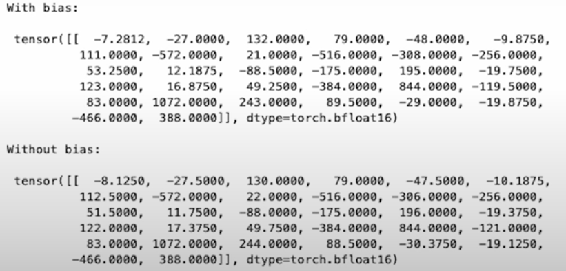

The W8A16linearLayer class:

The register buffer is the only option to store a buffer rather than a parameter, which means we don't need to compute gradients on that tensor; you can initialize it with whatever "dtype" you like.

class W8A16LinearLayer(nn.Module):
    def __init__(self, in_features, out_features, 
                 bias=True, dtype=torch.float32):
        super().__init__()
        self.register_buffer("int8_weights",torch.randint(-128, 127, (out_features, in_features), dtype=torch.int8))
        self.register_buffer("scales", torch.randn((out_features), dtype=dtype))
        if bias:
            self.register_buffer("bias", torch.randn((1, out_features), dtype=dtype))
        else:
            self.bias = None
def quantize(self, weights):
        w_fp32 = weights.clone().to(torch.float32)
        scales = w_fp32.abs().max(dim=-1).values / 127
        scales = scales.to(weights.dtype)
        int8_weights = torch.round(weights/scales.unsqueeze(1)).to(torch.int8)
        self.int8_weights = int8_weights
        self.scales = scales
    
    def forward(self, input):
        return w8_a16_forward(self.int8_weights, input, self.scales, self.bias)      

module = W8A16LinearLayer(4, 8)
print("Weights before:\n" , module.int8_weights)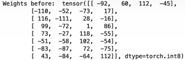

random_matrix = torch.randn((4, 8), dtype=torch.bfloat16)
module.quantize(random_matrix)
print("Weights After:\n" , module.int8_weights)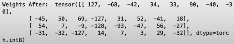

print(module.scales.shape) # torch.Size([4])
print(module.int8_weights.shape) # torch.Size([4,8])
dequentized_weights = module.int8_weights * module.scales.unsqueeze(1)
original_matrix = random_matrix
(original_matrix - dequentized_weights).abs().mean() # tensor(0.0045, dtpye=torch.bfloat16)

Replace PyTorch layers with Quantized Layers

We have all of the building blocks for our quantizer. Quantizer will cycle over all linear modules in your previous model, replacing them with our new W8A16 linear layer module and calling quantize with the original weights.

Model in-place linear layer replacement:

import torch
import torch.nn as nn
from helper import W8A16LinearLayer

def replace_linear_with_target(module, 
                               target_class, module_name_to_exclude):
    for name, child in module.named_children():
        if isinstance(child, nn.Linear) and not \
          any([x == name for x in module_name_to_exclude]):
            old_bias = child.bias
            new_module = target_class(child.in_features, 
                                      child.out_features, 
                                      old_bias is not None, 
                                      child.weight.dtype)
            setattr(module, name, new_module)
            if old_bias is not None:
              getattr(module, name).bias = old_bias
        else:
            # Recursively call the function for nested modules
            replace_linear_with_target(
                child, target_class, module_name_to_exclude)
class DummyModel(torch.nn.Module):
  def __init__(self):
    super().__init__()
    self.emb = torch.nn.Embedding(1, 1)
    # Try with bias
    self.linear_1 = nn.Linear(1, 1)
    # Try without bias
    self.linear_2 = nn.Linear(1, 1, bias=False)
    # Lm prediction head
    self.lm_head = nn.Linear(1, 1, bias=False)
model_1 = DummyModel()
model_2 = DummyModel()
replace_linear_with_target(model_1, W8A16LinearLayer, ["lm_head"])
print(model_1)
replace_linear_with_target(model_2, W8A16LinearLayer, [])
print(model_2)

Linear layer replacement and quantization:

def replace_linear_with_target_and_quantize(module, 
                               target_class, module_name_to_exclude):
    for name, child in module.named_children():
        if isinstance(child, nn.Linear) and not \
        any([x == name for x in module_name_to_exclude]):
            old_bias = child.bias
            old_weight = child.weight
            new_module = target_class(child.in_features, 
                                      child.out_features, 
                                      old_bias is not None, 
                                      child.weight.dtype)
            setattr(module, name, new_module)
            getattr(module, name).quantize(old_weight)
            
            if old_bias is not None:
              getattr(module, name).bias = old_bias
        else:
            # Recursively call the function for nested modules
            replace_linear_with_target_and_quantize(child, 
                     target_class, module_name_to_exclude)
model_3 = DummyModel()
replace_linear_with_target_and_quantize(model_3, W8A16LinearLayer, ["lm_head"])
print(model_3)

Quantize any Open Source PyTorch Model

Let’s try our custom quantizers on real models.

import torch
import torch.nn as nn
import torch.nn.functional as F
from helper import W8A16LinearLayer, replace_linear_with_target_and_quantize
from transformers import AutoModelForCausalLM, AutoTokenizer, pipeline
model_id = "./models/Salesforce/codegen-350M-mono"
model = AutoModelForCausalLM.from_pretrained(model_id, 
                                    torch_dtype=torch.bfloat16, 
                                    low_cpu_mem_usage=True)
tokenizer = AutoTokenizer.from_pretrained(model_id)
pipe = pipeline("text-generation", model=model, tokenizer=tokenizer)
print(pipe("def hello_world():", max_new_tokens=20, do_sample=False))
"""
[{'generated_text': 'def hello_world():\n    print("Hello World")\n\nhello_world()\n\n# 파'}]
"""
print("Model before:\n\n", model)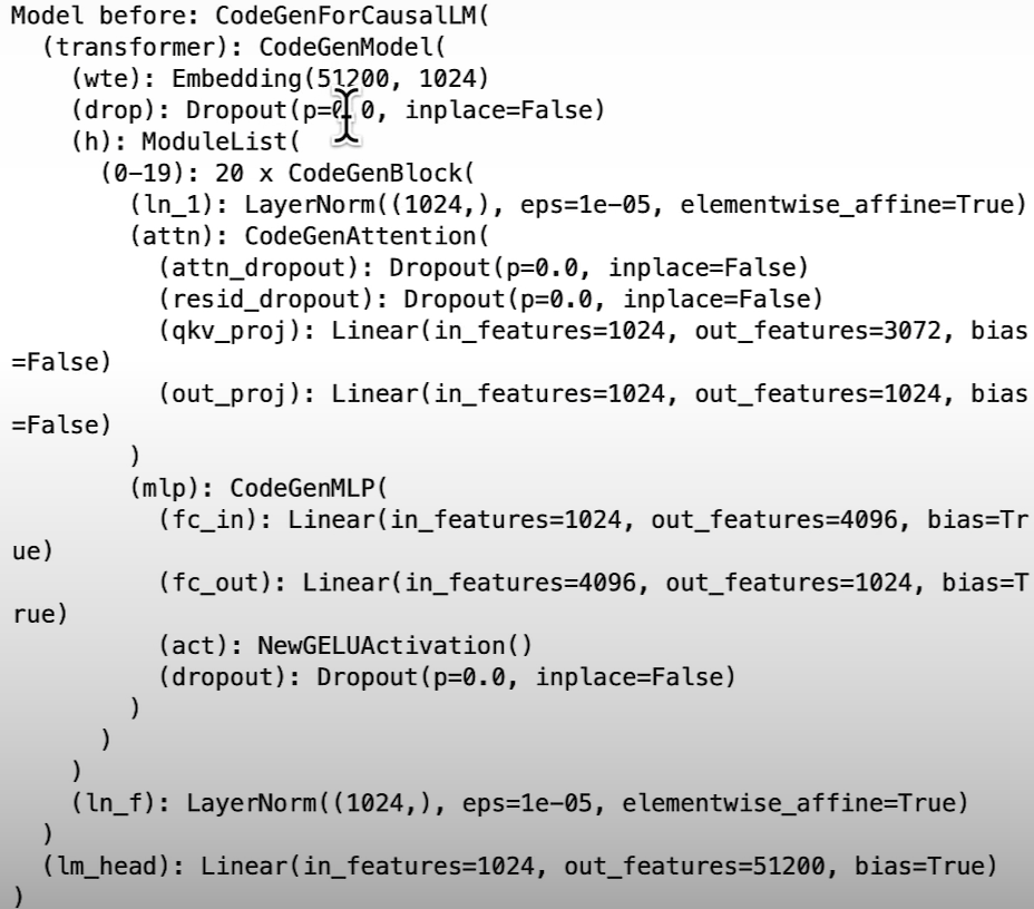

replace_linear_with_target_and_quantize(model, W8A16LinearLayer, ["lm_head"])
print(pipe.model)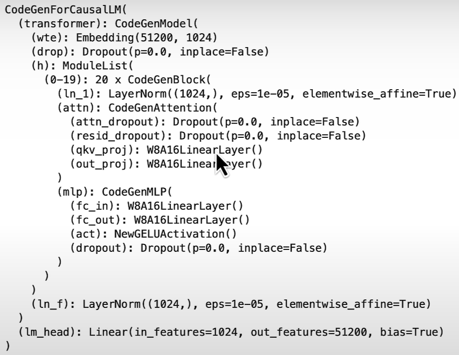

print(pipe("def hello_world():", max_new_tokens=20,do_sample=False)[0]["generated_text"])
"""
def hello_world():
    print("Hello World")
# hello_world()
# def hello_
"""

Let’s see how to call the quantizer on an object detection model. We will use Detr for object detection. Detr is an architecture that has been designed by Facebook AI and is used for object detection.

from transformers import DetrImageProcessor, DetrForObjectDetection
from PIL import Image
import requests
# you can specify the revision tag if you don't want the timm dependency
processor = DetrImageProcessor.from_pretrained("facebook/detr-resnet-50", revision="no_timm")
model = DetrForObjectDetection.from_pretrained("facebook/detr-resnet-50", revision="no_timm")
previous_memory_footprint = model.get_memory_footprint()
print("Footprint of the model in MBs: ", previous_memory_footprint/1e+6)
# Footprint of the model in MBs:  166.524032
img_path = "dinner_with_friends.png"
image = Image.open(img_path).convert("RGB")
image

from helper import plot_results
inputs = processor(images=image, return_tensors="pt")
with torch.no_grad():
  outputs = model(**inputs)
# convert outputs (bounding boxes and class logits) to COCO API
# let's only keep detections with score > 0.9
target_sizes = torch.tensor([image.size[::-1]])
results = processor.post_process_object_detection(outputs, target_sizes=target_sizes, threshold=0.9)[0]
plot_results(model, image, results)

print(model)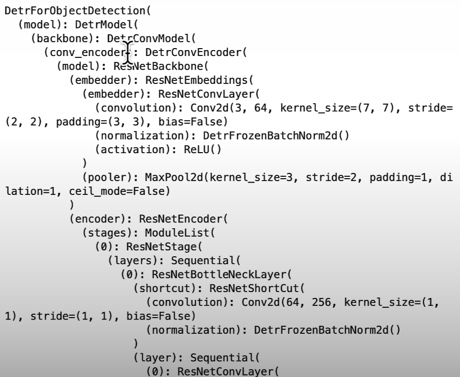

replace_linear_with_target_and_quantize(model, W8A16LinearLayer,[“0”, “1”, “2”, “class_labels_classifier”])
### Model after quantization
print(model)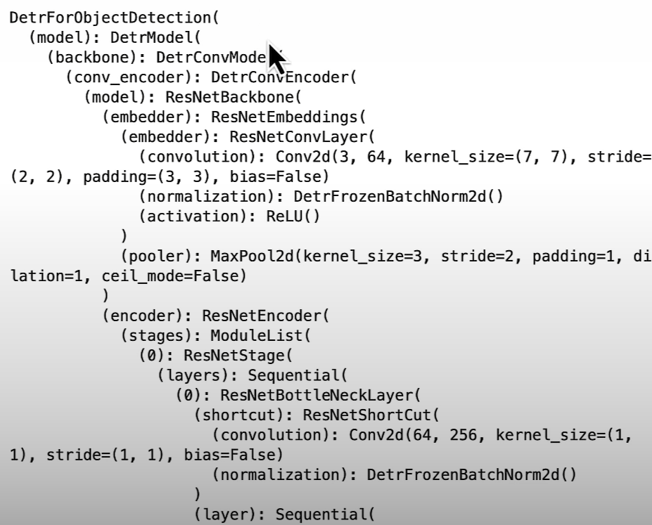

inputs = processor(images=image, return_tensors=”pt”)
with torch.no_grad():
 outputs = model(**inputs)
# convert outputs (bounding boxes and class logits) to COCO API
# let’s only keep detections with score > 0.9
target_sizes = torch.tensor([image.size[::-1]])
results = processor.post_process_object_detection(outputs, target_sizes=target_sizes, threshold=0.9)[0]
plot_results(model, image, results)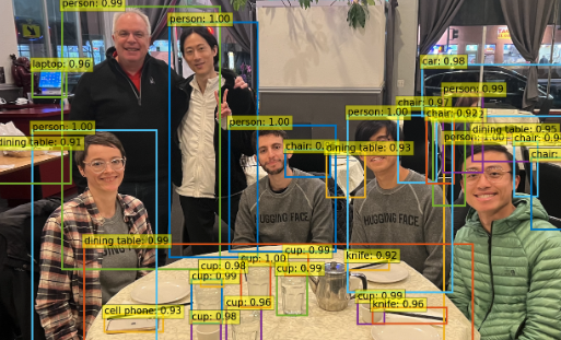

new_footprint = model.get_memory_footprint()
print("Footprint of the model in MBs: ", new_footprint/1e+6)
# Footprint of the model in MBs:  114.80384

### Memory saved
print("Memory saved in MBs: ", (previous_memory_footprint - new_footprint)/1e+6)
# Memory saved in MBs:  51.720192

Load your Quantized Weights from HuggingFace Hub

In the existing architecture, we must first load the model to its original precision before quantifying it. So, this is not ideal because you must dedicate enough RAM to load your model in the default d-type and then quantize it. In reality, you may be able to quantify the model by utilizing a large instance. If you have a powerful computing machine, you can quantize the model and then save the quantized weights elsewhere in the cloud. For example, connect to the HuggingFace hub and then load the model straight into your machine in 8-bit or lower accuracy.

The below example assumes we are on a high computation power machine.

import torch
from helper import W8A16LinearLayer, replace_linear_with_target_and_quantize, replace_linear_with_target
from transformers import AutoModelForCausalLM, AutoTokenizer

model_id = "./models/facebook/opt-125m"
model = AutoModelForCausalLM.from_pretrained(model_id, torch_dtype=torch.bfloat16, low_cpu_mem_usage=True)
tokenizer = AutoTokenizer.from_pretrained(model_id)
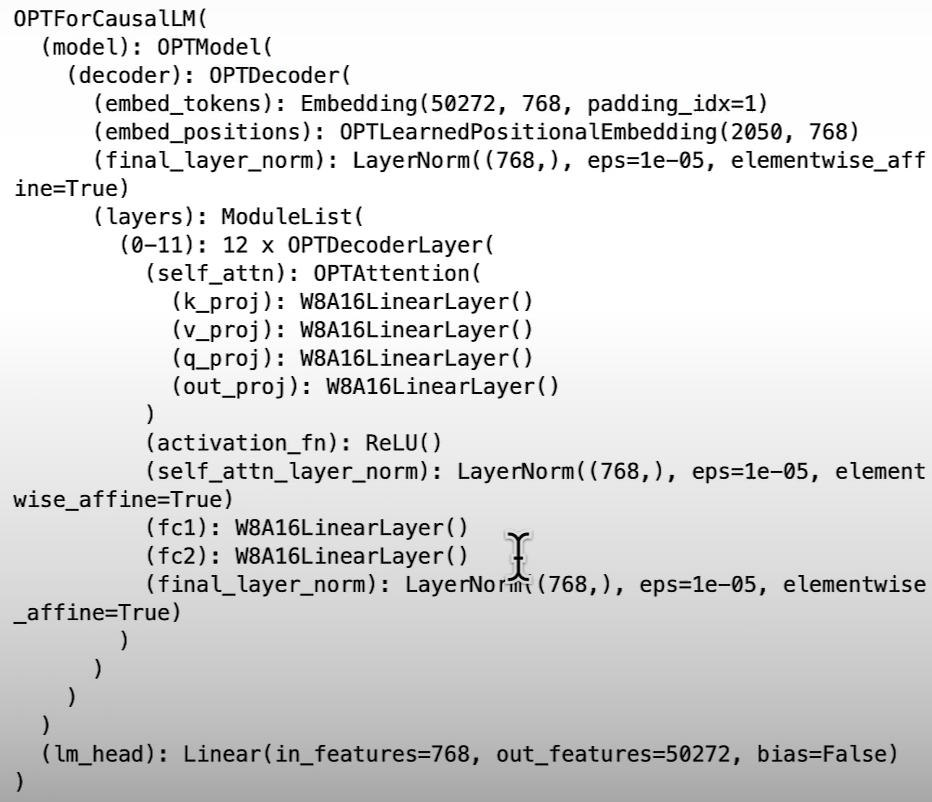
replace_linear_with_target_and_quantize(model, W8A16LinearLayer, ["lm_head"])
print(model)

quantized_state_dict = model.state_dict()
torch.save(quantized_state_dict, "quantized_state_dict.pth")

from huggingface_hub import HfApi, create_repo

YOUR_HF_USERNAME = ""
your_repo_id = f"{YOUR_HF_USERNAME}/opt-125m-quantized-dlai"

api = HfApi()

# create_repo(your_repo_id)

api.upload_file(
 path_or_fileobj="quantized_state_dict.pth",
 path_in_repo="quantized_state_dict.pth",
 repo_id=your_repo_id
)

We'll use the Pytorch meta device to load this model from HuggingFace. The goal here is to load the model's skeleton first to acquire the exact architecture, modules, and so on. And then, once we've loaded that skeleton, we simply need to replace all instances of linear layers with our quantized layers without quantizing the model, because we don't have access to the weights because they're all in the main device, so they're not being initialized. After you've changed all linear layers, simply call the model dot load state dict, passing the quantized state dict. 

The state dict will automatically apply the appropriate weights to each module. As a result, you save CPU RAM by not loading your original model. To begin, you load the quantized version of the model directly from the state dict. You're also using PyTorch's meta device, which allows you to load only the model's skeleton rather than the entire model.

To achieve this we first load the config of the model to get the details about the architecture of the model.

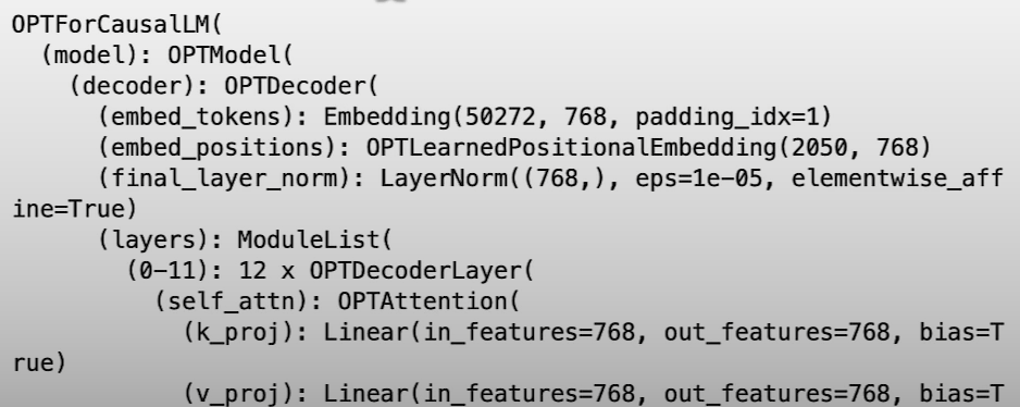
# Loading the model in meta device
from transformers import OPTForCausalLM, AutoTokenizer, AutoConfig

model_id = "./models/facebook/opt-125m"
config = AutoConfig.from_pretrained(model_id)

with torch.device("meta"):
  model = OPTForCausalLM(config)

tokenizer = AutoTokenizer.from_pretrained(model_id)
# Parameters have tensors but they are not initialized
for param in model.parameters():
  print(param) # Parameter containing: tensor(..., devide='meta', size=(50272, 768), required_grad=True)

print(model)

replace_linear_with_target(model, W8A16LinearLayer, ["lm_head"])
print(model)

from huggingface_hub import hf_hub_download

state_dict_cache_path = hf_hub_download(
    "ybelkada/opt-125m-quantized-dlai",
    "quantized_state_dict.pth"
)
state_dict = torch.load(state_dict_cache_path)
model.load_state_dict(state_dict, strict=True, assign=True)
# <All keys matched successfully>

Let’s try our quantized model:

from transformers import pipeline

pipe = pipeline("text-generation", model=model, tokenizer=tokenizer)
pipe("Hello today I am", max_new_tokens=40)
pipe = pipeline("text-generation", model=model, tokenizer=tokenizer)
pipe("Hello today I am giving a course about", max_new_tokens=10)

Weights Packing

Let's look at some common issues when using low-bit quantization, such as 2 or 4 bits, by going into weight spiking. Let's talk about why weight packing is crucial for storing quantized weights, how to store and load 2 and 4-bit weights in a packed uint8 tensor, and other issues when quantizing generative models like LLMS.

import torch
tensor = torch.tensor8[0,1], dtype=torch.int4) # NOT SUPPORTED
tensor = torch.tensor8[0,1], dtype=torch.uint8) # SUPPORTED BUT NOT IDEAL

Using 8-bit on Pytorch is not ideal because your tensor will occupy 8-bit per data point and might add a considerable overhead for large models (there would be no point quantizing to 2/4 bit).

To solve this we need to pack the 4-bit weights into 8-bit tensors. Consider the tensor below that stores 4 values that can be represented in 2-bit precision. In 2-bit precision, you can encode 4 values. In the case of base 2, we can encode 0123. We can code at most four values two to the power two.

import torch
tensor = torch.tensor([1,0,3,2], dtype=torch.uint8)
# Encoded as: 00000001 00000000 00000011 00000010

packed_tensor = torch.Tensor([177], dtype=torch.uint8)
# Encoded as: 10110001

Packing 2-Bit Weights

We use unsigned int instead of int8 because the first bit of an int8 tensor determines the tensor's sign. So, to keep things simple, instead of dealing with sign bits, we'll utilize unsigned bits.

# Example Tensor: [1, 0, 3, 2]
    # 1 0 3 2 - 01 00 11 10    
# Starting point of packed int8 Tensor
    # [0000 0000]    
##### First Iteration Start:
    # packed int8 Tensor State: [0000 0000]
    # 1 = 0000 0001
    # 0000 0001
    # No left shifts in the First Iteration
    # After bit-wise OR operation between 0000 0000 and 0000 0001:
    # packed int8 Tensor State: 0000 0001
    ##### First Iteration End    
##### Second Iteration Start:
    # packed int8 Tensor State: [0000 0001]
    # 0 = 0000 0000
    # 0000 0000
    # 2 left shifts:
    # [0000 0000] (1 shift)-> 0000 0000 (2 shift)-> 0000 0000
    # After bit-wise OR operation between 0000 0001 and 0000 0000:
    # packed int8 Tensor State: 0000 0001
    ##### Second Iteration End    
##### Third Iteration Start:
    # packed int8 Tensor State: [0000 0001]
    # 3 = 0000 0011
    # 0000 0011
    # 4 left shifts:
    # [0000 0011] (1 shift)-> 0000 0110 (2 shift)-> 0000 1100
    # 0000 1100 (3 shift)-> 0001 1000 (4 shift)-> 0011 0000
    # After bit-wise OR operation between 0000 0001 and 0011 0000:
    # packed int8 Tensor State: 0011 0001
    ##### Third Iteration End    
##### Fourth Iteration Start:
    # packed int8 Tensor State: [0011 0001]
    # 2 = 0000 0010
    # 0000 0010
    # 6 left shifts:
    # [0000 0010] (1 shift)-> 0000 0100 (2 shift)-> 0000 1000
    # 0000 1000 (3 shift)-> 0001 0000 (4 shift)-> 0010 0000
    # 0010 0000 (5 shift)-> 0100 0000 (6 shift)-> 1000 0000
    # After bit-wise OR operation between 0011 0001 and 1000 0000:
    # packed int8 Tensor State: 1011 0001
    ##### Fourth Iteration End
    # Final packed int8 Tensor State: [1011 0001

import torch
def pack_weights(uint8tensor, bits):
    if uint8tensor.shape[0] * bits % 8 != 0:
        raise ValueError(f"The input shape needs to be a mutiple of {8 / bits} - got {uint8tensor.shape[0]}")   
 num_values = uint8tensor.shape[0] * bits // 8
    num_steps = 8 // bits
    unpacked_idx = 0
    packed_tensor = torch.zeros((num_values), dtype=torch.uint8)
    
    # For each num_step (2 bits on the right) we will retrieve the corresponding value.
    # Next we will do bitwise shifting on the left for this tensor encoded in 8bits.
    # The shift will hapen bits * j times. Later bitwise or operation will be done on current packed tensor.
    
    """
    1 0 3 2 - 01 00 11 10
    [0000 0000] -> 0000 0001
    0000 0001
    0000 0000 - 0000 0000
    0000 0011 - 0011 0000 - 0011 0001
    1011 0001
    """
for i in range(num_values):
        for j in range(num_steps):
            packed_tensor[i] |= uint8tensor[unpacked_idx] << (bits * j)
            unpacked_idx += 1
    return packed_tensor
unpacked_tensor = torch.tensor([1, 0, 3, 2], dtype=torch.uint8)
pack_weights(unpacked_tensor, 2) # tensor([177], dtype=torch.uint8)
unpacked_tensor = torch.tensor([1, 0, 3, 2, 3, 3, 3, 3], dtype=torch.uint8)
pack_weights(unpacked_tensor, 2) # tensor([177, 255], dtype=torch.uint8)

Unpacking 2-Bit Weights

You need to unpack the weights to use them.

packed_tensor = torch.tensor([177], dtype=torch.uint8) # 10 11 00 01

We want to unpack them by extracting each 2-bit integer and assigning them into uint8 integers:

unpacked_tensor = torch.Tensor([1,0,3,2], dtype=torch.uint8) # 00000007 00000000 00000011 00000010

Algorithm Explanation:

# Example Tensor: [10110001]
    # Which was Originally: 1 0 3 2 - 01 00 11 10

    # Starting point of unpacked Tensor
    # [00000000 00000000 00000000 00000000]

    ##### First Iteration Start:
    # packed int8 Tensor: [10110001]
    # You want to extract 01 from [101100 01]
    # No right shifts in the First Iteration
    # After bit-wise OR operation between 00000000 and 10110001:
    # [10110001 00000000 00000000 00000000]
    # unpacked Tensor state: [10110001 00000000 00000000 00000000]
    ##### First Iteration End

    ##### Second Iteration Start:
    # packed int8 Tensor: [10110001]
    # You want to extract 00 from [1011 00 01]
    # 2 right shifts:
    # [10110001] (1 shift)-> 01011000 (2 shift)-> 00101100
    # After bit-wise OR operation between 00000000 and 00101100:
    # [10110001 00101100 00000000 00000000]
    # unpacked Tensor state: [10110001 00101100 00000000 00000000]
    ##### Second Iteration End

    ##### Third Iteration Start:
    # packed int8 Tensor: [10110001]
    # You want to extract 11 from [10 11 0001]
    # 4 right shifts:
    # [10110001] (1 shift)-> 01011000 (2 shift)-> 00101100
    # 00101100 (3 shift)-> 00010110 (4 shift)-> 00001011
    # After bit-wise OR operation between 00000000 and 00001011:
    # [10110001 00101100 00001011 00000000]
    # unpacked Tensor state: [10110001 00101100 00001011 00000000]
    ##### Third Iteration End

    ##### Fourth Iteration Start:
    # packed int8 Tensor: [10110001]
    # You want to extract 10 from [10 110001]
    # 6 right shifts:
    # [10110001] (1 shift)-> 01011000 (2 shift)-> 00101100
    # 00101100 (3 shift)-> 00010110 (4 shift)-> 00001011
    # 00001011 (5 shift)-> 00000101 (6 shift)-> 00000010
    # After bit-wise OR operation between 00000000 and 00000010:
    # [10110001 00101100 00001011 00000010]
    # unpacked Tensor state: [10110001 00101100 00001011 00000010]
    ##### Fourth Iteration End

    # Last step: Perform masking (bit-wise AND operation)
    # Mask: 00000011
    # Bit-wise AND operation between 
    # unpacked Tensor and 00000011
    # [10110001 00101100 00001011 00000010] <- unpacked tensor
    # [00000011 00000011 00000011 00000011] <- Mask
    # [00000001 00000000 00000011 00000010] <- Result

    # Final
    # unpacked Tensor state: [00000001 00000000 00000011 00000010]

def unpack_weights(uint8tensor, bits):
    num_values = uint8tensor.shape[0] * 8 // bits

    num_steps = 8 // bits

    unpacked_tensor = torch.zeros((num_values), dtype=torch.uint8)

    unpacked_idx = 0

    # 1 0 3 2 - 01 00 11 10

    # [00000000 00000000 00000000 00000000]
    # [10110001 00101100 00001011 00000010]
    # [00000001 00000000 00000011 00000010]

    # 10110001
    # 00000011
    
    # 00000001

    # 1: [10110001]
    # 2: [00101100]
    # 3: [00001011]

    mask = 2 ** bits - 1

    for i in range(uint8tensor.shape[0]):
        for j in range(num_steps):
            unpacked_tensor[unpacked_idx] |= uint8tensor[i] >> (bits * j)
            unpacked_idx += 1

    unpacked_tensor &= mask
    return unpacked_tensor


unpacked_tensor = torch.tensor([177, 255], dtype=torch.uint8)
unpack_weights(unpacked_tensor, 2) # Answer should be: torch.tensor([1, 0, 3, 2, 3, 3, 3, 3]

Beyond Linear Quantization

One of the most difficult aspects of quantization is dealing with the emergent properties of LLM. In 2022, researchers began to directly investigate the model's capabilities, discovering certain so-called emergent phenomena at scale. Emergen features are qualities or features that arise at scale in huge models.

For some models at scale, the features anticipated by the model, i.e. the size of the hidden states, began to grow huge, rendering traditional quantization strategies obsolete, resulting in conventional linear quantization algorithms failing on these models. Many researchers have decided to address the special difficulty of dealing with outlier features in LLMs. Outlier features merely indicate hidden states with a huge magnitude. There are other noteworthy articles, including Int8, SmoothQuant, and AWQ.

[https://huggingface.co/blog/hf-bitsandbytes-integration]

The matrix can be decomposed into two components. The outlier section includes all concealed stats that exceed a specific threshold, as well as the non-outlier part. So you quantize, multiply in eight bits, and then dequantize using the scales to get the final values in the input datatype. 

SmoothQuant's intuition: The activation X is difficult to quantify because outliers extend the quantization range, leaving only a few effective bits for most values. To lessen the difficulty of quantizing activations, we move the scale variance from them to weights W offline. The smoother activation X and the adjusted weight W are both easily quantifiable.

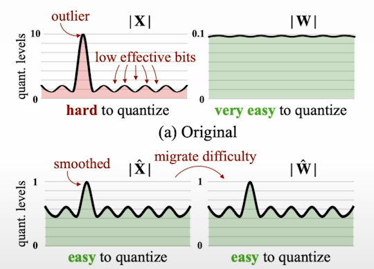
Another intriguing method is SmoothQuant. SmoothQuant is primarily applicable to A8W8 schemes. We also wish to quantify the activations. This indicates that both the activation and the weights have eight-bit precision. The research also addresses the issue of outliers in big language models. They proposed to alleviate this by smoothing both the activation and the weights. Given a factor determined based on the input activation, you can migrate the quantization complexity during both activation and weight quantization. 

So that's where you distribute the quantization difficulty evenly between the weights, as well as across the weights and the activation. This allows you to preserve the model's full capabilities.

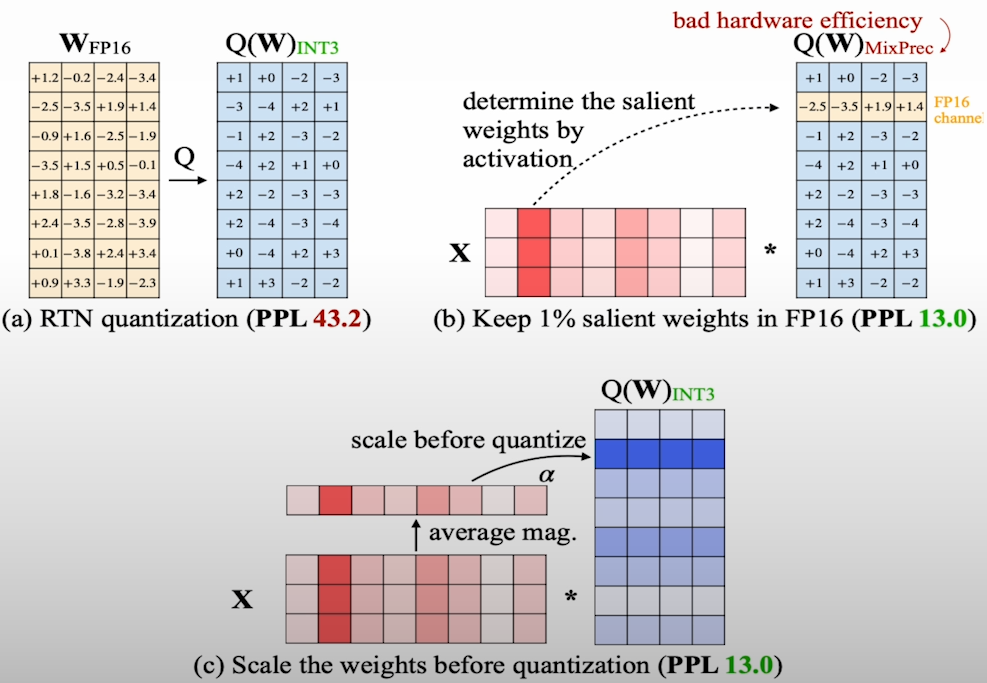
A more recent publication, AWQ, likewise addresses the outlier feature in a unique way. AWQ recommends iterating over a dataset, which we will refer to as a calibration dataset, to gain a deep understanding of which channel in the input weights is responsible for generating outlier features known as salient weights. The objective is to use that knowledge to scale the model weights before to quantization, as well as rescale the input during inference.

Recent SOTA quantization methods (chronologically):

• LLM.INT8 (only 8-bit) — Aug 2022 Dettmers et al.
• GPTQ — Oct 2022 Frantar et al.
• SmoothQuant — Nov 2022 Xiao et al.
• QLoRA (only 4-bit) — May 2024 Dettmers et al.
• AWQ — June 2024 Lin et al.
• QuIP# (promising for 2-bit) July 2024 Tseng et al.
• HQQ (promising for 2-bit) November 2024 Badri et al.
• AQLM (promising for 2-bit) February 2024 Egiazarian et al.

Following are the one of the challenges of quantization because the models are very large:

• Retraining (Quantization Aware Training)
• Limited Hardware Support
• Calibration Dataset Needed
• Packing/Unpacking

For more:

• SoTA quantization papers
• MIT Han Lab
• Transformers quantization docs and blogposts
• llama.cpp discussions
• Reddit r/LocalLlama

Kaynaklar

[1] Deeplearning.ai, (2024), Quantization in Depth:

[https://www.deeplearning.ai/short-courses/quantization-in-depth/]