
The fourth part of the series that I started as a comprehensive guide to building and training neural networks with PyTorch.
Computer Vision and Convolutional Neural Networks
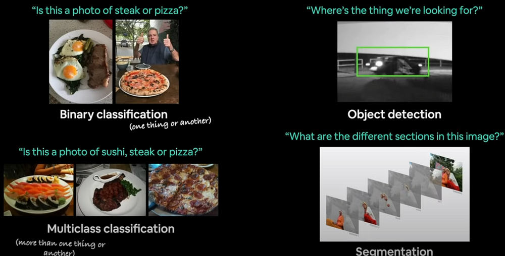
Computer vision is a branch of computer science that focuses on allowing computers to recognize and analyze visual data such as photos and movies.
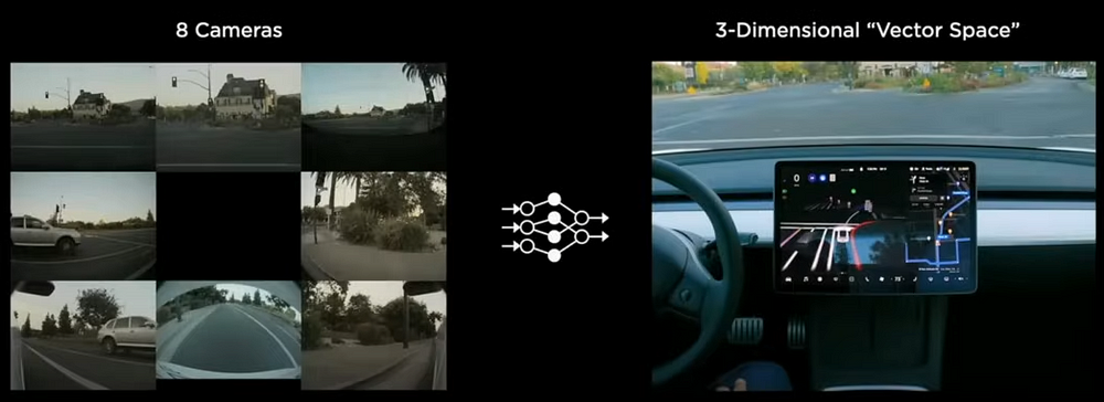
As shown here, self-driving cars construct a 3D model of their surroundings by combining images from cameras situated at various sites.
In this article, we will cover the following:
Working with a vision dataset with torch.vision.datasets
The CNN architecture in Pytorch.
End-to-end multiclass picture categorization challenge.
Steps for modelling with CNNs in PyTorch
Using Pytorch to create a CNN model, select a loss and optimizer, train the model, and then evaluate it.
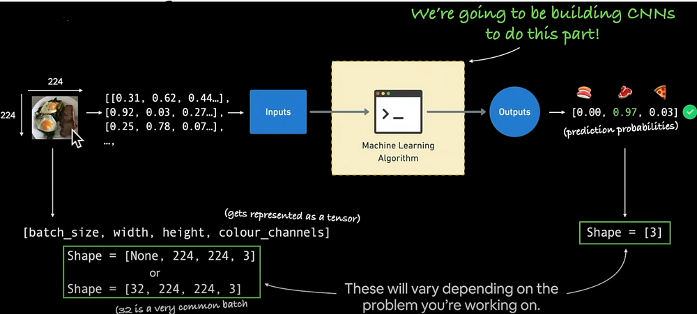
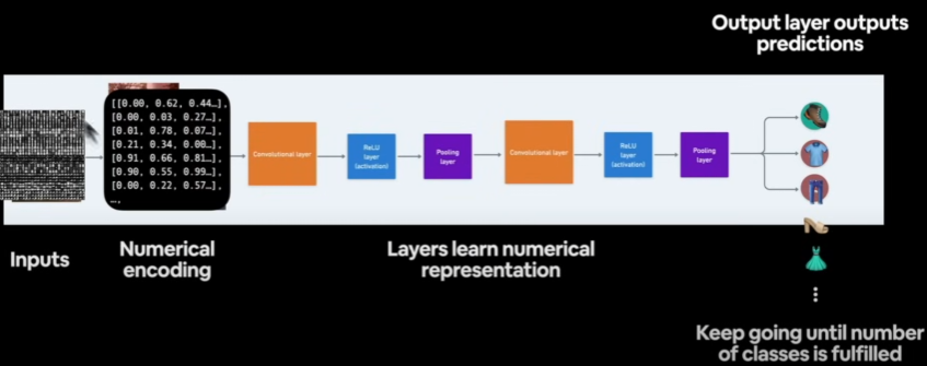
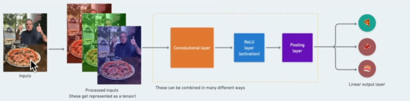
The following depicts how images are encoded. Images have height, width, colour channels (red, green, blue), and batch size (package size for each sending). We'll use Pytorch to create a deep-learning model called CNN. The output will feature three channels: sushi, steak, and pizza.
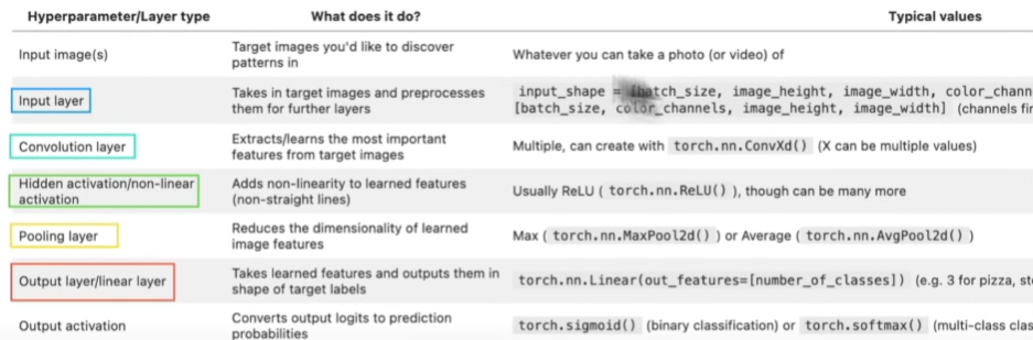
What is a Convolutional Neural Network (CNN)?
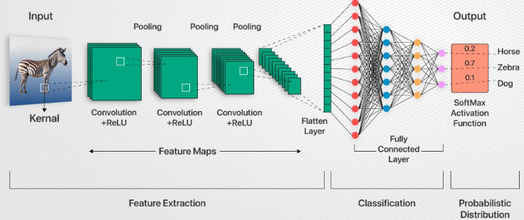
Convolutional neural networks, often known as ConvNets or CNNs, are deep learning network architectures that get their knowledge directly from data. When looking for patterns in photos to identify objects, classes, and categories, CNNs are quite helpful. They can also be very useful in the classification of signal data, time series, and audio.
- The Pytorch vision base domain library is called torchvision.
- torchvision.datasets Get computer vision datasets and data loading functions from this source.
- You can use computer vision models that have already been trained by torchvision.models to solve your own issues.
- Functions for modifying your vision data so that it may be used with Torch are provided by torchvision.transforms.utility.data.The Pytorch torch's base dataset class is called dataset.utility.data.Over a dataset, DataLoader generates a Python iterable.
import torch
from torch as nn

import torchvision
from torchvision import datasets
from torchvision import transforms
from torchvision.transforms import ToTensor

import matplotlib.pyplot as plt

# Below have different versions
print(torch.__version__)
print(torchvision.__version__)
Getting a dataset
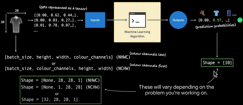
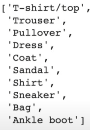
We will use FashionMNIST dataset from torchvision.datasets
A MNIST-like fashion product database. Benchmark :point_down: - GitHub - zalandoresearch/fashion-mnist: A MNIST-like…github.com
from torchvision import datasets
train_data  = datasets.FashionMNIST(
  root ="data", # where to download data
  train = True, # do we want the training dataset
  download = True, # do we want to download
  transform = torchvision.transform.ToTensor(), # how do we want to transform the data
  target_transform = None # how do we want to transform the labels/targets
)

test_data = datasets.FashionMNIST(
  root = "data",
  train = False,
  downloaded = True,
  transform = ToTensor(),
  target_transform = None
)print(train_data.class_to_idx)
print(train_data.classes)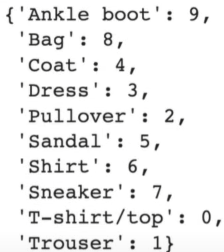
Let’s Visualize Our Data
import matplotlib.pyplot as plt
image, label = train_data[0]
plt.imshow(image.squeeze())
plt.title(label)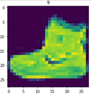
plt.imshow(image.squeeze(), cmap="grey")
plt.title(class_names[label])
plt.axis(False)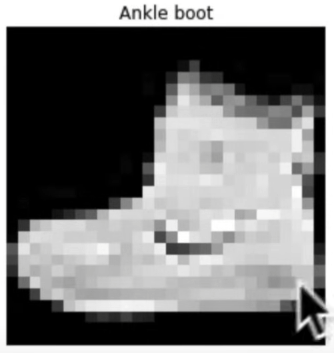
Let’s plot more data images to be one 🧘with the image:
torch.manual_seed(42)
fig = plt.figure(figsize=(9,9))
rows, cols = 4, 4
for i in range(1, rows*cols+1):
  random_idx = torch.randint(0, len(train_data), size=[1]).item()
  img, label = train_data[random_idx]
  fig.add_subplot(rows, cols, i)
  lt.imshow(img.squeeze(), cmap="gray")
  plt.title(class_names[labels])
  plt.axis(False)
Now let's get DataLoader ready:
Our data is currently available as Pytorch Datasets.
Our dataset is converted into a Python iterable via DataLoader.
Specifically, we would like to batch (or mini-batch) our data. Because hardware cannot handle all data at once, we take this action. Additionally, it increases the number of times our neural network may update its gradients inside each epoch.
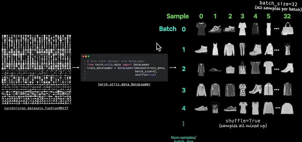
from torch.utils.data import DataLoader

BATCH_SIZE = 32

# Train data ise shuffle because we want our models to not learn order
train_dataloader = DataLoader(dataset=train_data,
                              batch_size=BATCH_SIZE,
                              shuffle=True)

train_dataloader = DataLoader(dataset=test_data,
                              batch_size=BATCH_SIZE,
                              shuffle=False)
Let’s check what we have created:
print(f"DataLoaders:{train_dataloader, test_dataloader}")
print(f"Length of train_dataloader:{len(train_dataloader) batches of {BATCH_SIZE}")
print(f"Length of test_dataloader:{len(test_dataloader) batches of {BATCH_SIZE}}")
What is inside the training dataloader?
train_features_batch, train_labels_batch = next(iter(train_dataloader))
train_features_batch.shape, train_labels_batch.shape
Model 0: Baseline Model
It's excellent practice to begin with a baseline model when developing a set of machine learning modeling trials. The baseline model is a basic model that you will attempt to enhance through other models and tests.
A continuous range of dims is flattened into a tensor via the flatten layer.
flatten_model = nn.Flatten()
x = train_features_batch[0]
output = flatten_model(x)
Let’s create the model:
from torch import nn
class FashionMNISTModelV0(nn.Module):
  def __init__(self,input_shape:int,hidden_units:int,output_shape:int):
    super().__init__()
    self.layer_stack = nn.Sequential(
      nn.Flatten(),
      nn.Linear(in_features=input_shape, out_features=hidden_units),
      nn.Linear(in_features=hidden_units, out_features=output_shape),
)

def forward(self, x):
  return self.layer_stack(x)
torch.manual_seed(42)
model_0 = FashionMNISTModelV0(
input_shape = 784, # 28 * 28
hidden_units = 10, # unit count in hidden layer
output_shpae = len(class_nmaes) # one for every class
).to("cpu")dummy_x = torch.rand([1, 1, 28, 28])
model_0(dummy_x)Now let's define the evaluation, optimizer, and loss metrics:
Given that we are utilizing multi-class data, nn will be our loss function.CorssEntropyClass
Our optimizer torch.optim.SGD()
Since we are working on a classification problem, let’s use accuracy as our evaluation metric.
import requests
from pathlib import Path

if not Path("helper_functions.py").is_file():
  request = request.get("https://raw.githubusercontent.com/mrdbourke/pytorch-deep-learning/main/helper_functions.py")
  with open("helper_functions.py","wb") as f:
    f.write(request.content)
from helper_functions import accuracy_fn
# Setup loss function and optimizer
loss_fn = nn.CrossEntropyLoss()
optimizer = torch.optim.SGD(params=model_0.parameters(), lr=0.1)Putting up a function to schedule our trials
The field of machine learning is highly experimental. Two primary variables that you should frequently monitor are the model's performance, which includes metrics like accuracy and loss, and its execution speed.
from timeit import default_timer() as timer
def print_train_time(start:float, end:float, device: torch.device = None):
  total_time = end - start
  print(f"Train time on {device}: {total_time:.3f} seconds")
  return total_time
start_time = timer()
end_time = timer()
print_train_time(start=start_time, end=end_time, device="gpu")Let's build a training loop and use data batches to train the model.
loop across epochs.
Calculate the training loss per batch, execute training steps, and then loop across training batches.
Calculate the test loss per batch, execute testing procedures, and then loop across testing batches.
Print out the current situation.
Time everything for enjoyment.
Take note: The loading bar visualization library for the console is called tqdm. The built-in Jupyter Notebook contains it.
from tqdm.auto import tqdm

torch.manual_seed(42)
train_time_start_on_cpu = timer()

# We will keep the epoch small for faster training time
epochs = 3

# Creating training and testing loop
for epoch in tqdm(range(epochs)):
  print(f"Epoch: {epoch}\n------")
  train_loss = 0
  for batch, (X, y) in enumerate(train_dataloader):
    model_0.train()
    y_pred = model_0(X) # forward pass
    # calculate loss per batch
    loss = loss_fn(y_pred, y)
    train_loss += loss # accumulate train loss

    optimizer.zero_grad()
    loss.backward()
    optimizer.step()

    if batch % 400 == 0:
      print(f"Looked at {batch * len(X)} / {len(train_dataloader.dataset)} samples.")

 # Divide total train loss by length of train dataloader
 train_loss /= len(train_dataloader)

 # Testing
 test_loss, test_acc = 0, 0
 model_0.eval()
 with torch.inference_mode():
  for X_test, y_test in test_dataloader:
    test_pred = model_0(X_test)

    test_loss += loss_fn(test_pred, y_test)

    test_acc += accuracy_fn(y_true=y_test, y_pred=test_pred.argmax(dim=1))

 test_loss /= len(test_dataloader)
 test_acc /= len(test_dataloader)

 print(f"Train loss: {train_loss:.4f} | Test loss: {test_loss:.4f}, Test ac: {test_acc:.4f}")

train_time_end_on_cpu = timer()
total_train_time_model_0 = print_train_time(start=train_time_start_on_cpu,
                                            end=train_time_end_on_cpu,
                                             device=str(next(model_0.parameters())))
Let’s make predictions:
torch.manual_seed(42)
def eval_model(modeL: torch.nn.Module,
               data_loader: torch.utils.data.DataLoader,
               loss_fn: torch.nn.Module,
               accuracy_fn,
               device = device):
"""Retruns a dictionary containing the results of model predicting on data_loader"""
loss, acc = 0, 0
model.eval()
with torch.inference_mode():
  for X, y in tqdm(data_loader):
    X, y = X.to(device), y.to(device)
    y_pred = model(X)
    loss += loss_fn(y_pred, y)
    acc += accuracy_fn(y_true=y, y_pred=y_pred.argmax(dim=1))
  loss /= len(data_loader)
  acc /= len(data_loader)

 return {"model_name": model.__class__.__name__, #only works when model was created with a class
         "model_loss": loss.item(),
         "model_acc": acc}

modeL-0_results = eval_model(model=model_0,
                             data_loader=test_dataloader,
                             loss_fn=loss_fn,
                              accuracy_fn=accuracy_fn)

model_0_results
Let's confirm if CUDA is being used by our GPU.
This terminal command displays the CUDA GPUs that are available:
!nvidia-smi
torch.cuda.is_available() # Return True or False
ModelV1: Building a better model with non-linearity
class FashionMNISTModelV1(nn.Module):
  def __init__(self, input_shape: int, hidden_units: int, output_shape:int):
    super().__init__()
    self.layer_stack = nn.Sequential(
      nn.Flatten(), # Flatten inputs into a single vector
      nn.Linear(in_features=input_shape, out_features=hidden_units),
      nn.ReLU(),
      nn.Linear(in_features=hidden_units, out_features=output_shape),
      nn.ReLU()
    )

  def forward(self, x:torch.Tensor):
    return self.layer_stac(x)

torch.manual_seed(42)
model_1 = FashionMNISTModelV1(input_shape=784, hidden_units=10, output_shape=len(class_names)).to(device)
next(model_1.parameters()).device()
Setup loss, optimizer and evaluation metrics
from helper_funcitons import accuracy_fn
loss_fn = nn.CrossEntropyLoss()
optimizer = torch.optim.SGD(params=model_1.parameters(), lr=0.1)
Functionalizing training and evaluation/testing loops
Let's write training loop testing_step() and training loop training_step() functions.
def train_step(modeL: torch.nn.Module,
               data_loader: torch.utils.data.DataLoader,
               loss_fn : torch.nn.Module,
               optimizer: torch.optim.Optimizer,
               accuracy_fn,
               device: torch.device = device):
"""Performs a training with model trying to learn on data_loader."""
train_loss, train_acc = 0, 0
model.train()
for batch, (X,y) in enumerate(data_Loader):
  X, y = X.to(device), y.to(device)
  y_pred = model(X)

  # Calculate loss and accuracy per batch
  loss = loss_fn(y_pred, y)
  train_loss += loss
  train_acc += accuracy_fn(y_true=y, y_pred=y_pred.argmax(dim=1)) # logits to prediction labels

  optimizer.zero_grad()
  loss.backward()
  optimizer.step()

  if batch % 400 == 0:
      printf(f"Looked at {batch * len(X)}/{len(train_dataloader.dataset)} samples.")

# Divide total train lsos and accuracy by length of train dataloader
train_loss /= len(train_dataloader)
train_acc /= len(data_loader)
printf(f"Train loss: {train_loss: .5f | Train acc: {train_acc: 2.f}%")
def test_step(model: torch.nn.Module,
data_loader: torch.utils.data.DataLoader,
loss_fn: torch.nn.Module,
accuracy_fn,
device: torch.device = device):
"""Performs a testing loop step on model going over data_loader."""
test_loss, test_acc = 0, 0
model.eval()
with torch.inference_mode():
for X, y in data_loader:
X, y = X.to(device), y.to(device)
test_pred = model(X)
test_loss += loss_fn(test_pred, y)
test_acc += accuracy_fn(y_true=y,y_pred=test_pred.argmax(dim=1))
# Adjust metrics and print out
test_loss /= len(data_loader)
test_acc /= len(data_loader)
printf(f"Train loss: {train_loss: .5f | Train acc: {train_acc: 2.f}%")torch.manual_seed(42)
from timeit import default_timer as timer
train_time_start_on_gpu = timer()
epochs = 3
for epoch in tqdm(range(epochs)):
printf(f"Epochs: {epoch}\n-------")
train_step(model=model_1,
data_loader=train_dataloader,
loss_fn=loss_fn,
optimizer=optimizer,
accuracy_fn=accuracy_fn,
device=device)
test_step(model=model_1,
data_loader=test_dataloader,
loss_fn=loss_fn,
accuracy_fn=accuracy_fn,
device=device)
train_time_end_on_gpu = timer()
total_train_time_model_1 = print_train_time(start=train_time_start,
end=train_time_end_on_gpu,
device=device)Caution: Depending on your hardware and data, your model may occasionally train more quickly on CPU than GPU.
This could be because the computing gains provided by the GPU are outweighed by the overhead associated with copying data/models to and from the GPU.
The CPU on the gear you're utilizing is more computationally capable than the GPU.
For more on how to make your models compute faster, see here: https://horace.io/brrr_intro.html
Let’s get model_1 results dictionary
model_1_results = eval_model(model = model_1,
                             data_loader = test_dataloader,
                             loss_fn = loss_fn,
                             accuracy_fn = accuracy_fn,
                             device = device)
Let’s build a convolutional neural network (CNN)
ConvNets are another name for CNNs. The capacity of CNNs to identify patterns in visual data is well recognized.

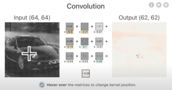
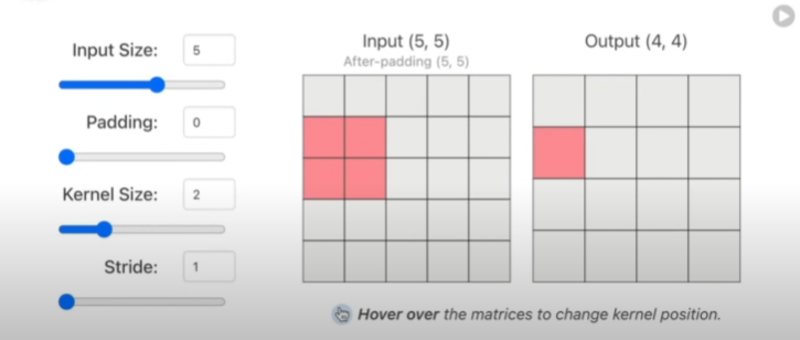
From the below address you can understand CNN better:
An interactive visualization system designed to help non-experts learn about Convolutional Neural Networks (CNNs).poloclub.github.io
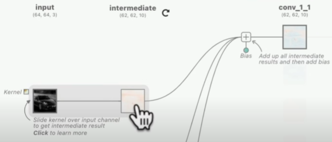
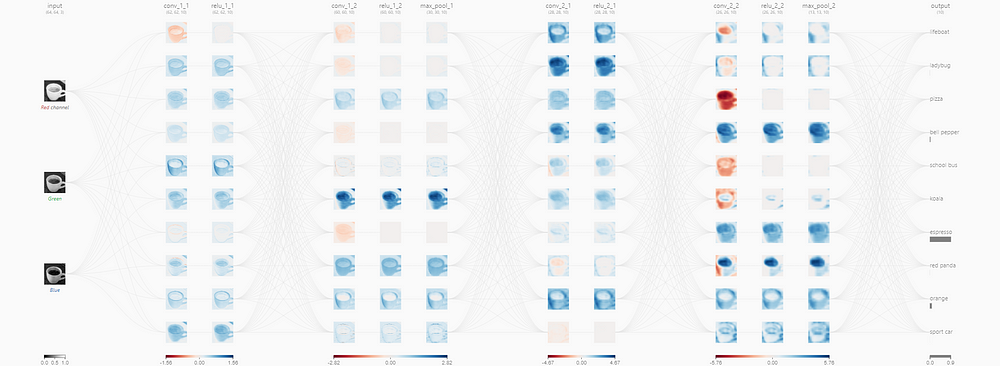
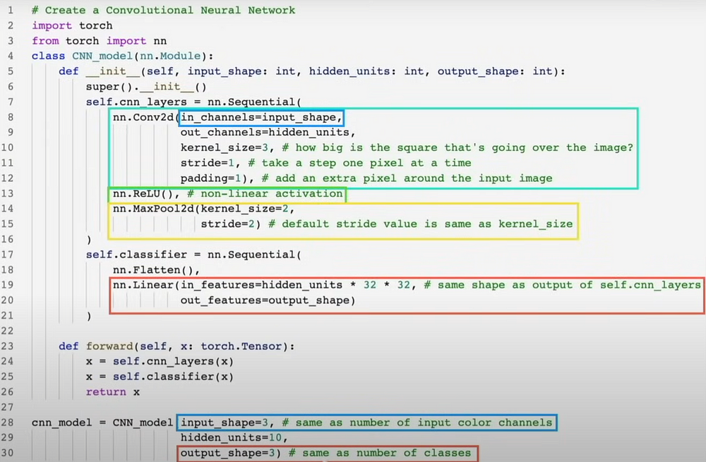
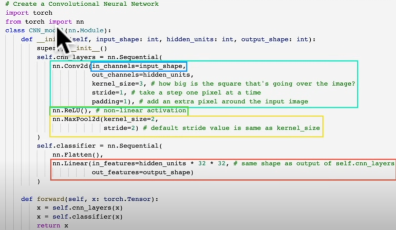
Let's create the deep learning layer in Pytorch mentioned above:
class FashionMNISTModelV2(nn.Module):
  "Model architecture that replicates the TinyVGG model from CNN explainer website."
  def __init__(self, input_shape: int, hidden_units: int, output_shape:int):
    super().__init__()
    self.conv_block_1 = nn.Sequential(
      nn.Conv2d(in_channels=input_shape,
                out_channels=hidden_units,
                kernel_size=3,
                stride=1,
                padding=1)
      nn.ReLU(),
      nn.Conv2d(in_channels=input_shape,
                out_channels=hidden_units,
                kernel_size=3,
                stride=1,
                padding=1),
      nn.ReLU(),
      nn.MaxPool2d(kernel_size=2)
)
  self.conv_block_2 = nn.Sequential(
      nn.Conv2d(in_channels=input_shape,
                out_channels=hidden_units,
                kernel_size=3,
                stride=1,
                padding=1)
      nn.ReLU(),
      nn.Conv2d(in_channels=input_shape,
                out_channels=hidden_units,
                kernel_size=3,
                stride=1,
                padding=1),
      nn.ReLU(),
      nn.MaxPool2d(kernel_size=2)
)
      self.classifier = nn.Sequential(
      nn.Flatten(),
      nn.Linear(in_features=hidden_units*0,
                out_features=output_shape)
)

def forward(self, x):
  x = self.conv_block_1(x)
  x = self.conv_block_2(x)
  x = self.classifier(x)
  return x
torch.manual_seed(42)
model_2 = FashionMNISTModelV2(input_shape=1, # input shape is 1 because there are no colors (e.g 3)
hidden_units=10,
output_shape=len(class_names),
kernel_size=(3,3),
stride=1,
padding=1)
conv_output = conv_layer(test_image.unsqueeze(0))
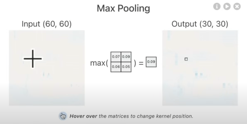
conv_output.shapeStepping through MaxPool2d()
max_pool_layer = nn.MaxPool2d(kernel_size=2)
test_image_through_conv = conv_layer(test_image.unsqueeze(dim=0))
test_image_through_conv_and_max_pool = max_pool_layer(test_image_through_conv)

print(test_image.shape)
print(test_image.unsqueeze(0).shape)
print(test_image_through_conv)
print(test_image_through_conv_and_max_pool)
Setup a loss function and optimizer for model_2
from helper_functions import accuracy_fn

loss_fn = nn.CrossEntropyLoss()
optimizer = torch.optim.SGD(params=model_2.parameters(), lr=0.2)
Training and testing model_2 using our training and test functions
torch.manuel_seed(42)
torch.cuda.manual_seed(42)

from timeit import default_timer as timer
train_time_start_model_2 = timer()

epochs = 3
for epoch in tqdm(range(epochs)):
  train_step(model=model_2,
             data_loader=train_dataloader,
             loss_fn=loss_fn,
             optimizer=optimizer,
             accuracy_fn=accuracy_fn,
             device=device)
  test_step(model=model_2,
            data_loader=test_dataloader,
            loss_fn=loss_fn,
            accuracy_fn=accuracy_fn,
            device=device)

  train_time_end_model_2 = timer()
  total_train_time_model_2 = print_train_time(start=train_time_start_model_2,
                                              end=train_time_end_model_2,
                                              device=device)
model_2_result= eval_model(
model=model_2,
data_loader=test_dataloader,
loss_fn=loss_fn,
accuracy_fn=accuracy_fn,
device=device
)Compare model results and training time
import pandas as pd
compare_results = pd.DataFrame([model_0_results, model_1,results, model_2_results])
compare_results["training_time"] = [total_train_time_model_0,
                                    total_train_time_model_1,
                                    total_train_time_model_2]
print(compare_results)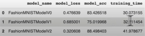
Make and evaluate random predictions with the best model
def make_predictions(model: torch.nn.Module, data: list, device: torch.device = device):
  pred_probs = []
  model.to(device)
  model.eval()
  with torch.inference_mode():
    for sample in data:
      sample = torch.unsqueeze(sample, dim=0).to(device)
      pred_logit = model(sample)
      pred_prob = torch.softmax(pred_logit.squeeze(), dim=0)
      pred_probs.append(pred_prob.cpu())

return torch.stack(pred.probs)
import random
random.seed(42)
test_sample=[]
test_labels = []
for sample, label in random.sample(list(test_data), k=9)
test_samples.append(sample)
test_samples.append(label)
plt.imshow(test_samples[0].squeeze(), cmap="gray")
plt.title(class_names[test_labels[0]])# Converting prediction probabilities to labels
pred_probs = make_predictions(model=model_2, data=test_samples)
pred_classes = pred_probs.argmax(dim=1)# Plot predictions
plt.figure(sigsize=(9,9))
nrows=3
ncols=3
for i, sample in enumerate(test_samples):
plt.subplot(nrows, ncols, i+1)
plt.imshow(sample.squeeze(), cmap="gray")
pred_label = class_names[pred_classes[i]]
truth_label = class_names[test_labels[i]]
title_text = f"Pred: {pred_label} | Truth : {truth_label}"
if pred_label == truth_label:
plt.title(title_text, fontsize=10, c="g")
else:
plt.title(title_text, fntsize=10, c="r")
plt.axis(False)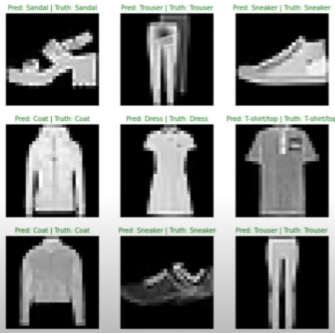
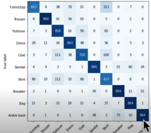
Confusion matrix creation for additional prediction assessment
An excellent visual evaluation tool for your classification models is a confusion matrix.
Using the test dataset, make predictions using our trained model.
Make a torchmetrics confusion matrix.
ConfusingMatrixUtilizing mlxtend.plotting.plot_confusion_matrix(), plot the confusion matrix
import tqdm.auto import tqdm

# Make predicitons with trained model
y_preds = []
model_2.eval()
with torch.inference_mode():
  for X, y in tqdm(test_dataloader, desc="Making predictions..."):
    # Send data and targets to target device
    X, y = X.to(device), y.to(device)
    y_logit = model_2(X)
    # Turn predictions from logits to predicition probabilities to prediction labels
    y_preds = torch.softmax(y_logits.squeeze(), dim=0).argmax(dim=1)
    #Put prediction on CPU for evaluation
    y_preds.append(y_pred.cpu())

# Concatenate list of predictions into a tensor
y_pred_tensor = torch.cat(y_preds)


try:
  import mlxtend, torchmetrics
  assert int(mlxtend.__version__.split(".")[1]) >= 19, "mlextend version should be 0.19.0 or higher")
except:
  !pip install -q torchmetrics -U mlxtend
  import torchmetrics, mlxtend
from torchmetrics import ConfusionMatrix
from mlxtend.plotting import plot_confusion_matrix
confmat = ConfusionMatrix(num_classes=len(class_names))
confmat_tensor = confmat(preds=y_pred_tensor, target=test_data.targets)
fig, ax = plot_confusion_matrix(conf_mat=confmat_tensor.numpy(),
class_names=class_names,
figsize=(10,7)
)
Saving and loading our model
from pathlib import Path

MODEL_PATH = Path("models")
MODEL_PATH.mkdir(parents=True, exist_ok=True)

MODEL_NAME = "computer_vision_model.pth"
MODEL_SAVE_PATH = MODEL_PATH / MODEL_NAME

print(f"Saving the model to:{MODEl_SAVE_PATH}")
torch.save(obj=model_2.state_dict(), f=MODEL_SAVE_PATH)
image_shape = [1, 28, 28]
torch.manual_seed(42)
loaded_model_2 = FashionMNISTModelV2(input_shape=1,
hidden_unit=10,
output_shape=len(class_names))
loaded_model_2.load_state_dict(torch.load(f=MODEL_SAVE_PATH))
loaded_model_2.to(device)Evaluating loaded model
torch.manual_seed(42)

loaded_model_2_results = eval_model(
  model=loaded_model_2,
  data_loader=test_dataloader,
  loss_fn=loss_fn,
  accuracy_fn=accuracy_fn
)
Verifying if the model's output is reasonably near to one another
torch.isclose(torch.tensor(model_2_results["model_loss"]),
  torch.tensor(loaded_model_2_results["model_loss"]),
  atol=1e-02)
Resource
[1] freeCodeCamp.org, (6 Ekim 2022), PyTorch for Deep Learning & Machine Learning — Full Course:


0 Comments