
https://cbarkinozer.medium.com/pytorch-ustal%C4%B1k-serisi-b%C3%B6l%C3%BCm-3-4b78206b543f
The third part of the series that I started as a comprehensive guide to building and training neural networks with PyTorch.
Neural Network Classification
Classification is the process of putting objects into groups or classes based on their similarities and affinities, and it expresses the unity of attributes that may exist among a diverse range of persons.
For example, identifying email spam is a binary classification challenge. Multiclass classification is the process of categorizing images based on their content. Documents can be classed by adding tags; known as multi-label categorization.
What we will discuss:
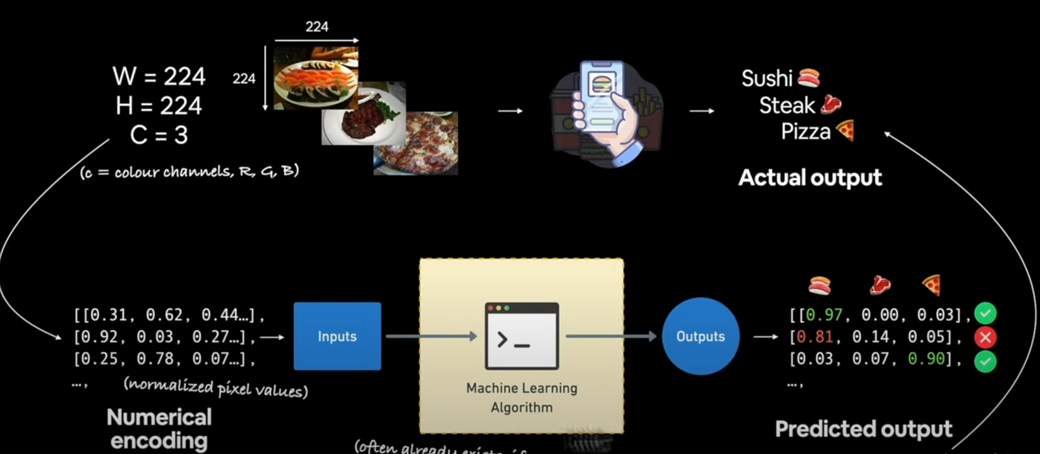
Neural Network Classification model architecture.
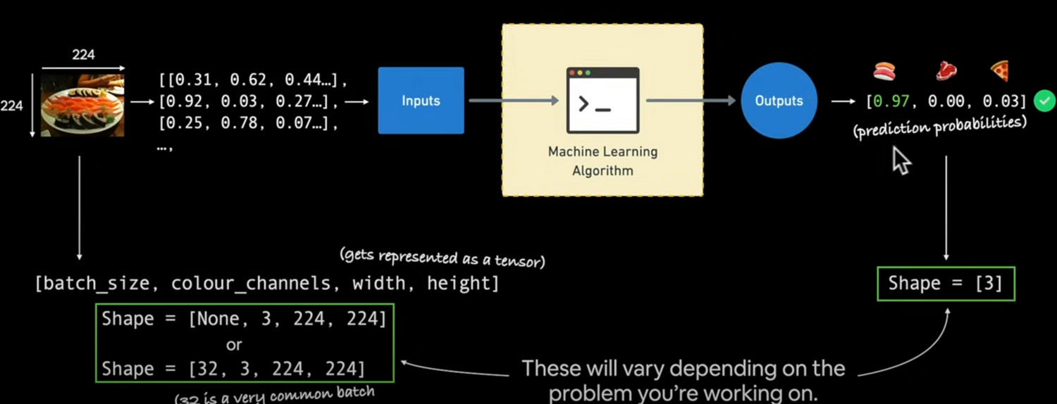
The input and output shapes of a classification model.
Creating custom data for viewing, fitting, and predicting.
Modelling steps include building a model, specifying a loss function and optimiser, establishing a training loop, and assessing the model.
Saving and loading models.
Using the power of nonlinearity.
Various categorization evaluation procedures.
Let's create classification data and get it ready.
import sklearn
from sklearn.datasets import make_circles

n_samples = 1000

X,y = make_circles(n_samples, noise = 0.03, random_state = 42)

print(len(X)) # 1000
print(len(y)) # 1000

print(X[:5])
print(y[:5])

# Make dataframe from circle data

import pandas as pd
circles = pd.DataFrame({"X1":X[:,0],"X2":X[:,1],"label":y})
circles.head(10)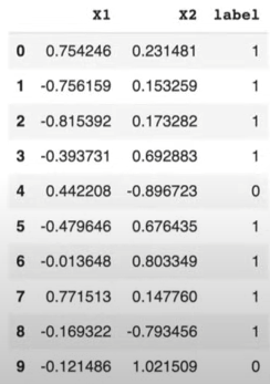
import matplotlib.pyplot as plt
plt.scatter(x=X[:,0],y=X[:,1],c=y,cmap=plt.cm.RdY1Bu)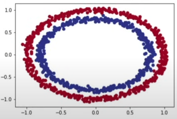
Let's convert the data into tensors and generate train and test divides.
import torch
X = torch.from_numpy(X).type(torch.float)
y = torch.from_numpy(y).type(torch.float)

torch.manual_seed(42)

from sklearn.model_selection import train_test_split # splits train and test randomly
X_train, X_test, y_train, y_test = train_test_split(X, y, test_size=0.2)
Let's create a model that distinguishes between blue and red dots. We'll set up a GPU, build a model, specify the loss function and optimizer, and develop a training and testing loop.
import torch
from torch import nn

device = "cuda" if torch.cuda.is_available() else "cpu"
Now that we've defined device-agnostic code, let's build a model that
- Subclass ‘nn.Module’ (like almost all models).
- Create 2 ‘nn.Linear()’ layers that are capable of handling the shapes of our data.
- Defines a ‘forward()’ method that outlines the forward pass.
- Instantiate an instance of our model class and send it to the target ‘device’.
class CircleModelV0(nn.Module):
  def __init__(self):
    super().__init__()
    self.layer_1 = nn.Linear(in_features=2, out_features=5) # takes 2 features and upscales to 5 features
    self.layer_2 = nn.Linear(in_features=5, out_features=5) # takes 5 features from previous layer and outputs a single feature (same shape as y)

  def forward(self, x):
    return self.layer_2(self.layer_1(x)) # x -> layer_1 -> layer_2 -> output

model_0 = CircleModelV0().to(device)
The categorization playground below allows you to see how a neural network works:
https://playground.tensorflow.org/
If you are using simpler ways like the above CircleModelV0, you may also use the following method:
model_0 = nn.Sequential(
  nn.Linear(in_features=2,out_features=5),
  nn.Linear(in_features=5,out_features=1)
).to(device)
or mix both like this:
class CircleModelV0(nn.Module):
  def __init__(self):
    super().__init__()
    self.two_linear_layers = nn.Sequential(
      nn.Linear(in_features=2,out_features=5),
      nn.Linear(in_features=5,out_features=1)
    )

def forward(self, x):
    return two_linear_layers(x)

model_0 = CircleModelV0().to(device)
Make predictions:
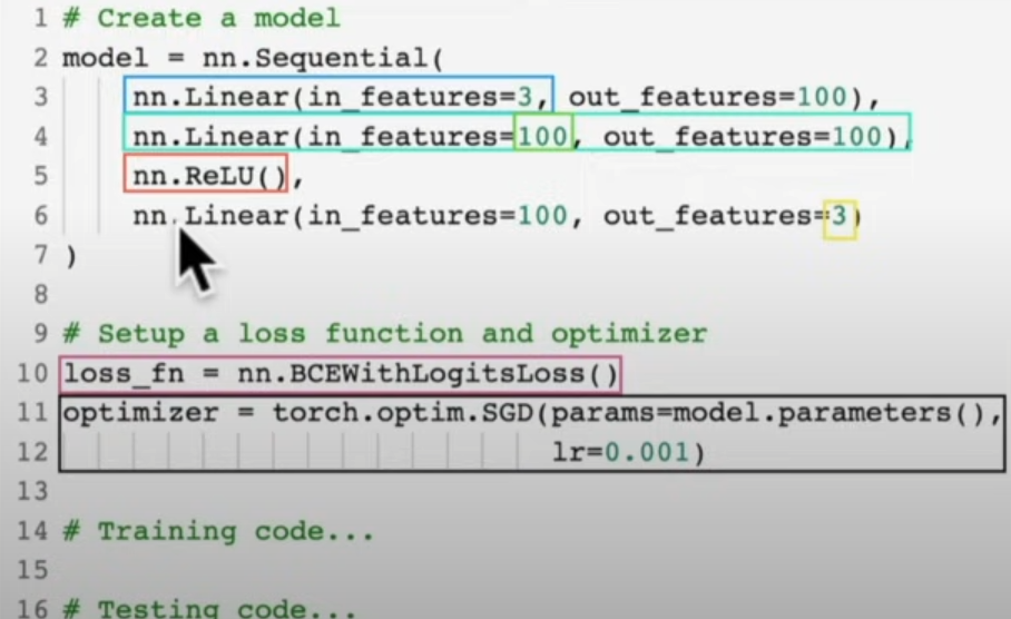
untrained_preds = model_0(X_test.to(device))For categorization, you might use binary or categorical cross-entropy. For the loss function, we'll use 'torch.nn.BECWithLogitsLoss()'.
Let us calculate accuracy. We seek accuracy, which is the absolute truth. Accuracy is calculated using this formula:
Accuracy = True Positive / (True Positive + True Negative) * 100
def accuracy(y_true, y_pred):
  correct = torch.eq(y_true, y_pred).sum().item()
  acc = (correct/len(y_pred)) * 100
  return acc
Our model's outputs will be logits. Logits are the model's raw, unnormalized predictions made before adding any activation function. We may turn these logits into prediction probabilities by sending them through an activation function (such as sigmoid for binary classification or softmax for multiclass classification).
Logits -> prediction probabilities -> prediction labels
The prediction probabilities in our model can then be converted to prediction labels by rounding or using the argmax() method.
model_0.evaluation()
with torch.inference_mode():
  y_logits = model_0(X_test.to(device))[:5]

y_pred_probs = torch.sigmoid(y_logits)
We need to apply a range-style rounding on our prediction probability values.
y_pred_probs ≥0.5, y=1 (class 1)
y_pred_probs <0.5, y=0 (class 0)
# Find the predicted labels
y_preds = torch.round(y_pred_probs)

# In full (logits -> pred probs -> pred labels)
y_pred_labels = torch.round(torch.sigmoid(model_0(X_test.to(device))[:5]))

# Check for equality
print(torch.eq(y_preds.squeeze(), y_pred_labels.squeeze()))

# Get rid of extra dimensions
y_preds.squeeze()
Building a training and testing loop
torch.manuel_seed(42)
torch.cuda.manuel_seed(42)
epochs = 100
X_train, y_train = X_train.to(device), y_train.to(device)
X_test, y_train = X_test.to(device), y_Test.to(device)
# Training and testing loop
for epoch in range(epochs):
model_0.train()
# Forward Pass
y_logits = model_0(X_train).squeeze()
y_pred = torch.round(torch.sigmoid(y_logits))
# Calculate Loss/Accuracy
loss = loss_fn(y_logits, y_train)
acc = accuracy_fn(y_true=y_train, y_pred=y_pred)
optimizer.zero_grad()
loss.backward() # backpropagation
optimizer.step() # gradient descend
model_0.eval()
with torch.inference_mode():
test_logits = model_0(X_test).squeeze()
test_pred = torch.round(torch.sigmoid(test_logits))
test_loss = loss_fn(test_logits, y_test)
test_acc = accuracy_fn(y_true= y_test, y_pred=test_pred)
if epoch % 10 == 0:
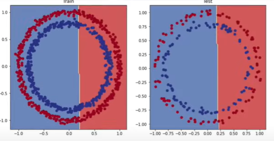
print(f"Epoch: {epoch}, Loss: {loss:.5f}, Accuracy: {acc.2f}%, Test Loss:{test_loss.5f}, Test Accuracy: {test_acc.2f}%")After running the aforementioned code, we can see that our model isn't learning. To gain a better understanding, let's depict the predictions. Let's import the plot_decision_boundary() method.
import requests
from pathlib import Path

if Path("helper_functions.py").is_file():
  pass
else:
  request = requests.get("https://raw.githubusercontent.com/mrdbourke/pytorch-deep-learning/")
  with open("helper_functions.py","wb") as f:
    f.write(request.content)

from helper_functions import plot_predictions, plot_decision_boundary

plt.figure(figsize=(12,6))
plt.subplot(1,2,1)
plt.train("Train")
plot_decision_boundary(model_0, X_train, y_train)
plt.subplot(1,2,2)
plt.title("Test")
plot_decision_boundary(model_0,X_test,y_test)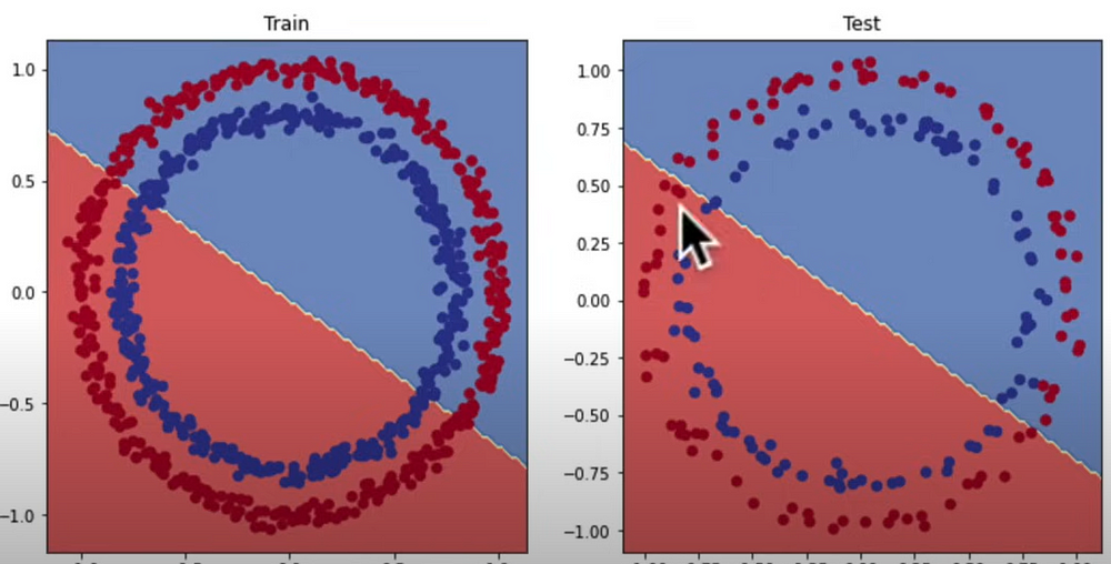
How can we increase the model's performance?
- Adding more layers increases the model's ability to learn about patterns in the data.
Adding more hidden units (it is normally recommended to use 5 to 10 hidden layers in this level of difficulty).
Be fit for longer.
Adjusting the activation functions.
Change the learning rate (learning does not occur if it is too small, and gradients burst if it is too great).
Data can also be changed via preprocessing (e.g., eliminating NaN values).
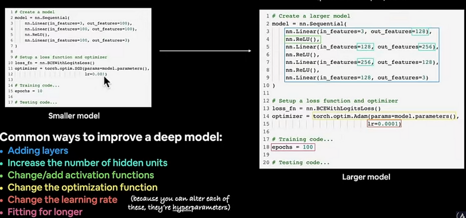
!Experiment Tracking Tip: Make these modifications gradually so you can determine which changes have the greatest positive impact on the outcome.
Despite these adjustments, we are still unable to build an effective clustering.
We replace the dataset with our prior regression one and discover that our model has no trouble learning; the issue is with the dataset.
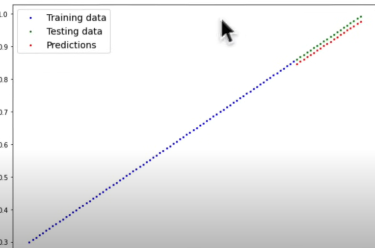
The difficulty was that our model predicted using linear lines when we needed nonlinearity.
Building a model with non-linearity
from torch import nn

class CircleModelV2(nn.Module):
  def __init__(self):
    super().__init__()
    self.layer_1 = nn.Linear(in_features=2,out_features=10)
    self.layer_2 = nn.Linear(in_features=10,out_features=10)
    self.layer_3 = nn.Linear(in_features=10,out_features=1)
    self.relu = nn.Relu()
    self.sigmoid = nn.Sigmoid()

def forward(self, x):
    return self.layer_3(self.relu(self.layer_2(self.relu(self.layer_1(x)))))

model_2 = CircleModelV2().to(device)

loss_fn = nn.BCEWithLogitsLoss()
optimizer = torch.optim.SGD.(model_3.parameters(), lr=0.1)

torch.manual_seed(42)
torch.cuda.manual_seed(42)

X_train, y_train = X_train.to(device), y_train.to(device)
X_test, y_test = X_test.to(device), y_test.to(device)

epochs = 1000

for epoch in range(epochs):
  model_2.train()
  y_logits = model_3(X_train).squeeze()
  y_pred = torch.round(torch.sigmoid(y_logits))

  loss = loss_fn(y_logits, y_train)
  acc = accuracy_fn(y_true=y_train, y_pred = y_pred)

  optimizer = zero_grad()
  loss.backward()

  optimizer.step()

  model_2.eval()
  with torch.inference_mode():
    test_logits = model_2(X_Tests).squeeze()
    test_pred = torch.round(torch.sigmoid(test_logits))

    test_loss = loss_fn(test_logits, y_test)
    test_acc = accuracy_fn(y_true = y_test, y_pred = test_pred)

  if epoch % 100 == 0:
    print(f"Epoch: {epoch}, Loss: {loss:.5f}, Accuracy: {acc.2f}%, Test Loss:{test_loss.5f}, Test Accuracy: {test_acc.2f}%")
More parameters improve learning ability, but they reduce training and inference speed and need more computing power.
Let us assess the correctness of our model using a non-linear activation function:
model_2.eval()
with torch.inference_mode():
  y_preds = torch.round(torch.sigmoid(model_2(X_test))).squeeze()

plt.figure(figsize = (12,6))
plt.subplot(1, 2, 1)
plt.title("Train")
plot_decision_boundry(model_3, X_train, y_train)
plt.subplot(1, 2, 1)
plt.title("Test")
plot_decision_boundary(model_3, X_test, y_test)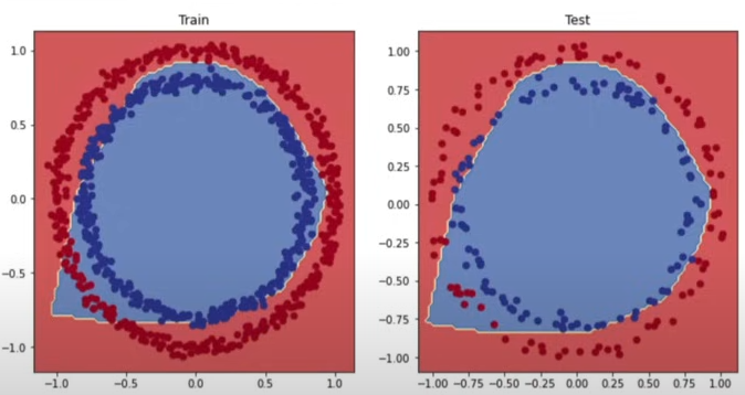
The output quality is fairly good, notwithstanding a minor inaccuracy in the lower left features.
The output quality is fairly good, with the exception of a minor irregularity in the bottom left corner.
Multiclass Classification
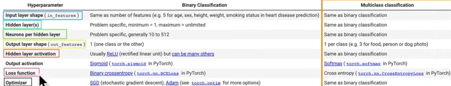
Multiclass classification is the process of classifying more than two classes.
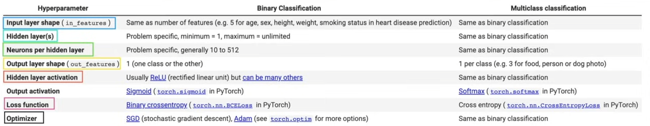
In multiclass classification, some hyperparameters, such as output layer geometry, hidden layer activation, output activation, loss function, and optimizer, differ from those in binary classification.
import torch
import matplotlib.pyplot as plt
import sklearn.datasets import make_blobs # toy dataset
import sklearn.model_selection import train_test_split

NUM_CLASSES = 4
NUM_FEATURES = 2
RANDOM_SEED = 42

X_blob, y_blob = make_blobs(n_samples = 1000,
                            n_features = NUM_FEATURES,
                            centers = NUM_CLASSES,
                            cluster_std = 1.5,
                            random_state= RANDOM_SEED)

X_blob = torch.from_numpy(X_blob).type(torch.float)
y_blob = torch.from_numpy(y_blob).type(torch.LongTensor)

X_blob_train, X_blob_test, y_blob_train, y_blob_test = train_test_split(X_blob, y_blob,test_size=0.2,random_state=RANDOM_SEED)

plt.figure(figsize=(10,7))
plt.scatter(X_blob[:,0], X_blob[:,1], c=y_blob, cmap=plt.cm.RdYlBu)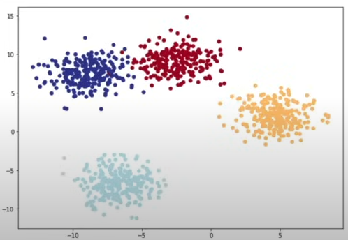
Building the multiclass classification model
device = "cuda" if torch.cuda.is_available() else "cpu"

class BlobModel(nn.Module):
  def __init__(self, input_features, output_features, hidden_units=8):
    super().__init__()
    self.linear_layer_stack = nn.Sequential(
      nn.Linear(in_features=input_features, out_features=hidden_units),
      nn.ReLU(),
      nn.Linear(in_features=hidden_units, out_features=hidden_units),
      nn.ReLU(),
      nn.Linear(in_features=hidden_units, out_features=output_features)
    )

 def forward(self, x):
    return self.linear_layer_stack(x)

model_3 = BlobModel(input_features=2, output_features=4, hidden_units=8).to(device)
Creating a loss function and optimizer for a multiclass example
loss_fn = nn.CrossEntropyLoss()

optimizer = torch.optim.SGD(params=model_3.parameters(), lr=0.1)
Predicting results
To evaluate, test, and train our model, we must first transform its outputs to prediction probabilities, followed by prediction labels.
model_3.eval()
witch torch.inference_mode():
  y_preds = model_3(X_blob_test.to(device))

y_pred_probs = torch.softmax(y_logits, dim=1)
# Convert our model's prediction probabilities to prediction label
y_preds = torch.argmax(y_pred_probs, dim=1)
Creating a training and testing loop
torch.manual_seed(42)
torch.cuda.manual_seed(42)
epochs=100

X_blob_train, y_blob_train = X_blob_train.to(device), y_blob_train.to(device)
X_blob_test, y_blob_test = X_blob_test.to(device), y_blob_test.to(device)

for epoch in range(epochs):
  model_3.train()

  y_logits = model_3(X_blob_train)
  y_pred = torch.softmax(y_logits, dim=1).argmax(dim=1)

  loss = loss_fn(y_logits, y_blob_train)
  acc = accuracy_fn(y_true= y_blob_train, y_pred=y_pred)

  optimizer.zero_grade()
  loss.backward()
  optimizer.step()

  model_3.eval()

  with torch.inference_mode():
    test_logits = model_3(X_blob_test)
    test_preds = torch.softmax(test_logits, dim=1).argmax(dim=1)

    test_loss = loss_fn(test_logits, y_blob_test)
    test_acc = accuracy_fn(y_true=y_blob_test, y_pred = test_preds)


  if epoch % 100 == 0:
    print(f"Epoch: {epoch}, Loss: {loss:.5f}, Accuracy: {acc.2f}%, Test Loss:{test_loss.5f}, Test Accuracy: {test_acc.2f}%")
Evaluating Predictions
model_3.eval()

  with torch.inference_mode():
    y_logits = model_3(X_blob_test)

y_pred_probs = torch.softmax(y_logits, dim=1)

plt.figure(figsize=(12,6))
plt.subplot(1,2,1)
plt.title("Train")
plot_decision_boundary(model_3, X_blob_train, y_blob_train)
plt.subplot(1,2,1)
plt.title("Test")
plot_decision_boundary(model_3, X_blob_test, y_blob_test)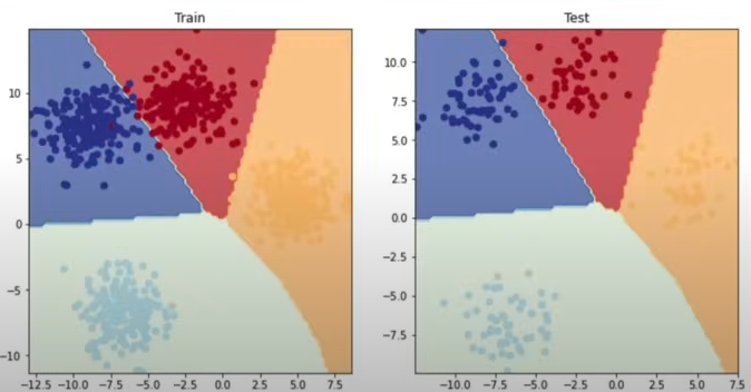
If we eliminated the ReLU layers from our ANN, it would still work in this case since our elements are linearly separable; however, if our elements were non-linearly separable (such as pizza components), it would fail.
Classification Metrics

To evaluate the model's performance in classification issues, a variety of measures can be used. Some of the most widely used measures are:
1. Accuracy
The accuracy metric measures how many of the model's total predictions are correct. Its formula is tp+tn / (tp+tn+fp+fn).
Code:
import torchmetrics
accuracy = torchmetrics.Accuracy()
2. Precision
The precision metric measures how many of the examples the model predicts as positive are actually positive. Its formula is tp / (tp+fp).
import torchmetrics
precision = torchmetrics.Precision()
3. Recall
The recall metric measures how much of the examples the model correctly predicts are actually positive. Its formula is tp / (tp+fn).
import torchmetrics
recall = torchmetrics.Recall()
4. F1-score
The F1-score metric is the harmonic mean of precision and recall. Its formula is 2 * (precision * recall) / (precision + recall).
import torchmetrics
f1_score = torchmetrics.F1Score()
5. Confusion Matrix
The complexity matrix metric visualizes the relationship between the model's predictions and the actual labels. Can be created using torchmetrics.ConfusionMatrix().
import torchmetrics
confusion_matrix = torchmetrics.ConfusionMatrix()
Let’s calculate the accuracy of our model:
!pip install torchmetrics

from torchmetrics import Accuracy

torchmetric_accuracy = Accuracy().to(device)

torchmetric_accuracy(y_preds, y_blob_test)
Reference
[1] freeCodeCamp.org, (6 Ekim 2022), PyTorch for Deep Learning & Machine Learning — Full Course:


0 Comments