Vector Databases: from Embeddings to Applications

https://medium.com/@cbarkinozer/vekt%C3%B6r-veritabanlar%C4%B1-yerle%C5%9Ftirmelerden-uygulamalara-c2b1e23909c2

An overview of Deeplearning.ai's "Vector Databases: from Embeddings to Applications" course.

LLMs fall short when a new or different data source is requested. To overcome this retrieval problem, an enhanced generation strategy is developed, and RAG employs vector databases. Vector databases allow you to search by semantics (meaning) rather than syntax (letter combinations).

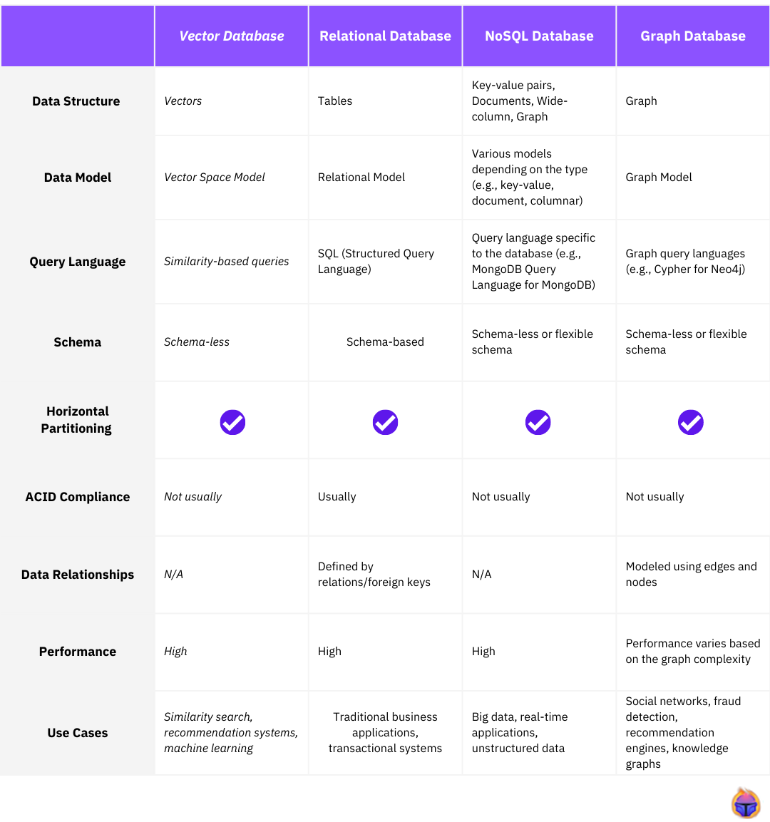
Here's a database-type comparison:

Weaviate sponsored this episode. Weaviate is an open-source, AI-powered vector database that can aid. AI-powered applications are created by developers to be intuitive and dependable.

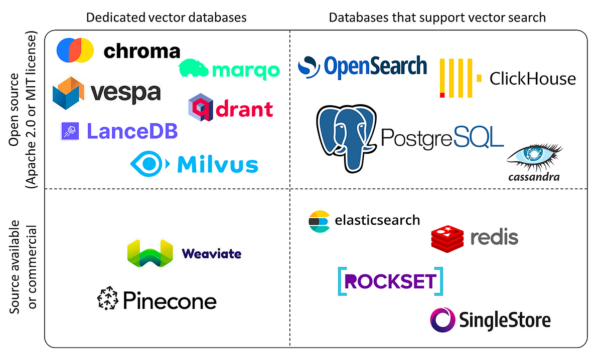
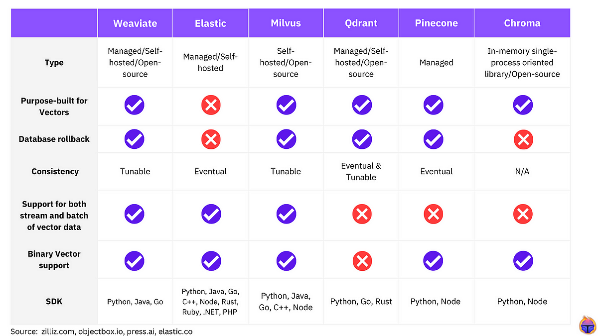
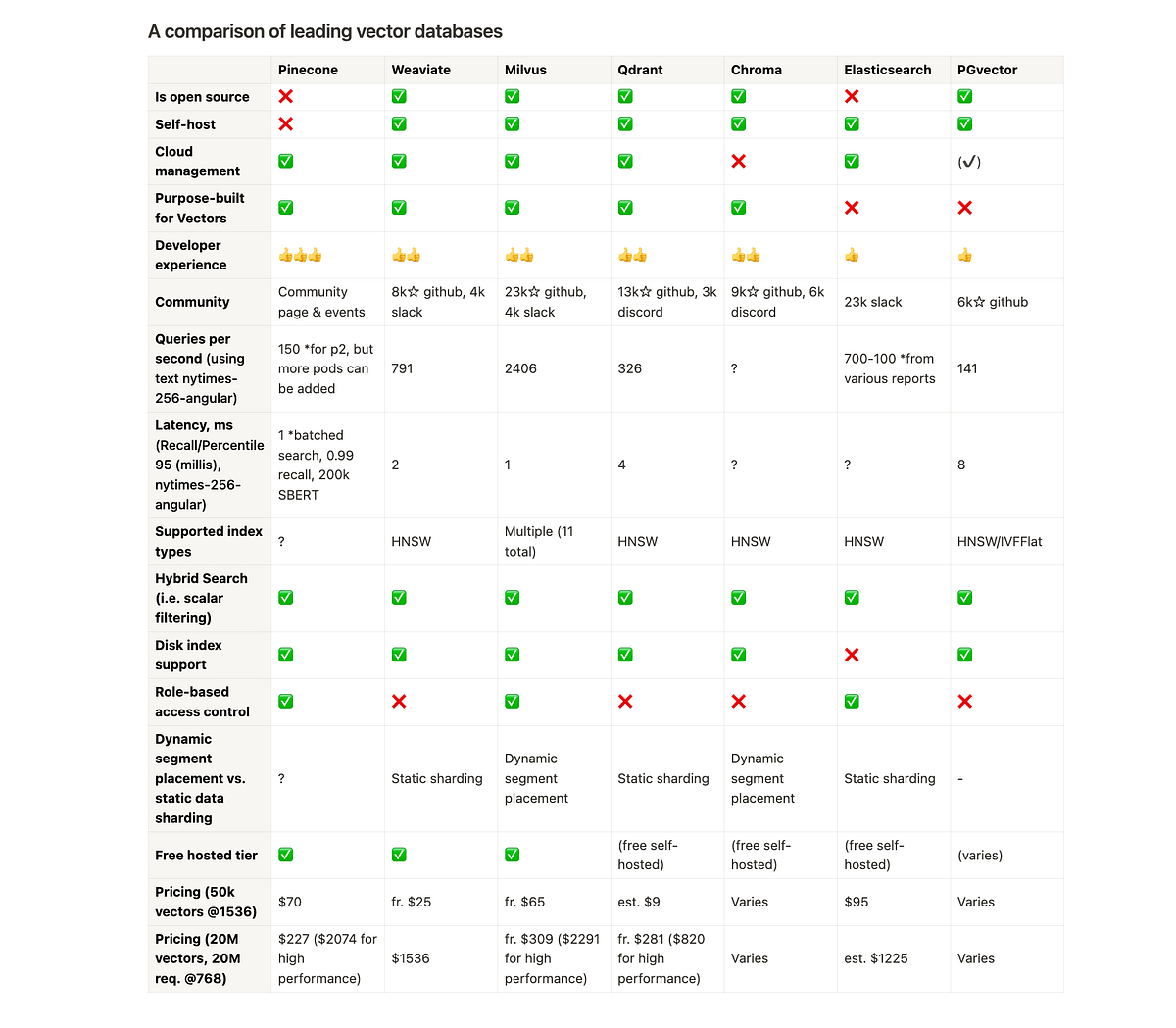
Here's a comparison of some vector databases:

Contents of the course

• Embeddings
• Distance Metrics
• ANN — Trade recall for accuracy
• HNSW
• CRUD operations
• Objects+vectors
• Inverted index — filtered search
• ANN search over Dense embeddings
• Sparse search
• Hybrid search
• VectorDB implementations in the industry

How to obtain vector representations of data?

Large language models typically convert photos, videos, text, or other data sources into float numbers known as vectors. This operation is known as embedding. Embedding occurs because huge language networks can determine where they fit in their semantic (meaning) space. Understanding football and soccer image/video/text is highly comparable, however basketball and swimming content are less similar.

How can we measure the distance between these Image and Sentence Embeddings?

There are several methods for calculating the distance between two vectors.

In this section, we will look at four distance measures that are commonly employed in vector databases:

• Euclidean Distance(L2): The length of the shortest path between two points or vectors.

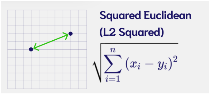
# Euclidean Distance
L2 = [(zero_A[i] - zero_B[i])**2 for i in range(len(zero_A))]
L2 = np.sqrt(np.array(L2).sum())
print(L2)

#An alternative way of doing this
np.linalg.norm((zero_A - zero_B), ord=2)

#Calculate L2 distances
print("Distance zeroA-zeroB:", np.linalg.norm((zero_A - zero_B), ord=2))
print("Distance zeroA-one:  ", np.linalg.norm((zero_A - one), ord=2))
print("Distance zeroB-one:  ", np.linalg.norm((zero_B - one), ord=2))

• Manhattan Distance(L1): Distance between two points if one was constrained to move only along one axis at a time.

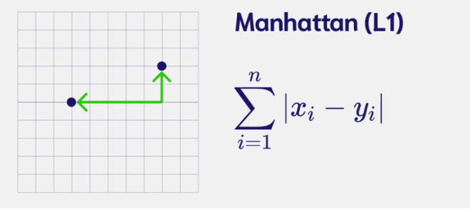
# Manhattan Distance
L1 = [zero_A[i] - zero_B[i] for i in range(len(zero_A))]
L1 = np.abs(L1).sum()

print(L1)

#an alternative way of doing this is
np.linalg.norm((zero_A - zero_B), ord=1)

#Calculate L1 distances
print("Distance zeroA-zeroB:", np.linalg.norm((zero_A - zero_B), ord=1))
print("Distance zeroA-one:  ", np.linalg.norm((zero_A - one), ord=1))
print("Distance zeroB-one:  ", np.linalg.norm((zero_B - one), ord=1))

• Dot Product: Measures the magnitude of the projection of one vector onto the other.

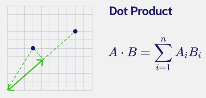
# Dot Product
np.dot(zero_A,zero_B)

#Calculate Dot products
print("Distance zeroA-zeroB:", np.dot(zero_A, zero_B))
print("Distance zeroA-one:  ", np.dot(zero_A, one))
print("Distance zeroB-one:  ", np.dot(zero_B, one))

• Cosine Distance: Measure the difference in directionality between vectors.

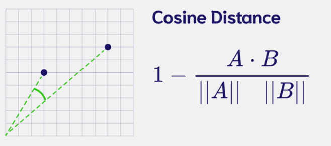
# Cosine Distance
cosine = 1 - np.dot(zero_A,zero_B)/(np.linalg.norm(zero_A)*np.linalg.norm(zero_B))
print(f"{cosine:.6f}")

zero_A/zero_B

# Cosine Distance function
def cosine_distance(vec1,vec2):
  cosine = 1 - (np.dot(vec1, vec2)/(np.linalg.norm(vec1)*np.linalg.norm(vec2)))
  return cosine

#Cosine Distance
print(f"Distance zeroA-zeroB: {cosine_distance(zero_A, zero_B): .6f}")
print(f"Distance zeroA-one:   {cosine_distance(zero_A, one): .6f}")
print(f"Distance zeroB-one:   {cosine_distance(zero_B, one): .6f}")

Search for similar vectors

The brute force KNN method is the default search algorithm for vector databases.

KNN, or the K nearest neighbour algorithm, simply looks around a vector to find its K nearest neighbour. The nearness is calculated using the Euclidean distance, which we discussed earlier.

Brute force search algorithm:

1. Measure the L2 distance between the query and each vector.
2. Sort all those distances.
3. Return the top k matches. These are the most semantically similar points.

Brute force search has O(dN) runtime complexity for search.

K Nearest Neighbour Implementation:

import numpy as np
import matplotlib.pyplot as plt
from sklearn.neighbors import NearestNeighbors
import time
np.random.seed(42)

# Generate 20 data points with 2 dimensions
X = np.random.rand(20,2)

# Display Embeddings
n = range(len(X))

fig, ax = plt.subplots()
ax.scatter(X[:,0], X[:,1], label='Embeddings')
ax.legend()

for i, txt in enumerate(n):
    ax.annotate(txt, (X[i,0], X[i,1]))

k = 4

neigh = NearestNeighbors(n_neighbors=k, algorithm='brute', metric='euclidean')
neigh.fit(X)

# Display Query with data
n = range(len(X))

fig, ax = plt.subplots()
ax.scatter(X[:,0], X[:,1])
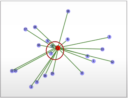
ax.scatter(0.45,0.2, c='red',label='Query')
ax.legend()

for i, txt in enumerate(n):
    ax.annotate(txt, (X[i,0], X[i,1]))

neighbours = neigh.kneighbors([[0.45,0.2]], k, return_distance=True)
print(neighbours)

t0 = time.time()
neighbours = neigh.kneighbors([[0.45,0.2]], k, return_distance=True)
t1 = time.time()

query_time = t1-t0
print(f"Runtime: {query_time: .4f} seconds")

def speed_test(count):
    # generate random objects
    data = np.random.rand(count,2)
    
    # prepare brute force index
    k=4
    neigh = NearestNeighbors(n_neighbors=k, algorithm='brute', metric='euclidean')
    neigh.fit(data)

    # measure time for a brute force query
    t0 = time.time()
    neighbours = neigh.kneighbors([[0.45,0.2]], k, return_distance=True)
    t1 = time.time()

    total_time = t1-t0
    print (f"Runtime: {total_time: .4f}")

    return total_time

Results:

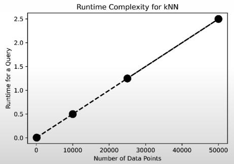
# Brute force examples (seconds)
time20k = speed_test(20_000) # 0.0030
time200k = speed_test(200_000) # 0.0095
time2m = speed_test(2_000_000) # 0.0144
time20m = speed_test(20_000_000) # 0.1171
time200m = speed_test(200_000_000) # 12.7856

Brute-force KNN implementation:

documents = 1000
dimensions = 768

embeddings = np.random.randn(documents, dimensions) # 1000 documents, 768-dimensional embeddings
embeddings = embeddings / np.sqrt((embeddings**2).sum(1, keepdims=True)) # L2 normalize the rows, as is common

query = np.random.randn(768) # the query vector
query = query / np.sqrt((query**2).sum()) # normalize query

# kNN
t0 = time.time()
# Calculate Dot Product between the query and all data items
similarities = embeddings.dot(query)
# Sort results
sorted_ix = np.argsort(-similarities)
t1 = time.time()

total = t1-t0
print(f"Runtime for dim={dimensions}, documents_n={documents}: {np.round(total,3)} seconds")

print("Top 5 results:")
for k in sorted_ix[:5]:
    print(f"Point: {k}, Similarity: {similarities[k]}")

n_runs = [1_000, 10_000, 100_000, 500_000]

for n in n_runs:
    embeddings = np.random.randn(n, dimensions) #768-dimensional embeddings
    query = np.random.randn(768) # the query vector
    
    t0 = time.time()
    similarities = embeddings.dot(query)
    sorted_ix = np.argsort(-similarities)
    t1 = time.time()

    total = t1-t0
    print(f"Runtime for 1 query with dim={dimensions}, documents_n={n}: {np.round(total,3)} seconds")

Result:

print (f"To run 1,000 queries: {total * 1_000/60 : .2f} minutes") 
# To run 1,000 queries: 31.38 minutes

This search time is not acceptable.

Approximate Nearest Neighbours (ANN)

KNN

The ANN algorithm uses a fraction of the accuracy of KNN to gain a lot of performance.

ANN

ANN implementation

from random import random, randint
from math import floor, log
import networkx as nx
import numpy as np
import matplotlib as mtplt
from matplotlib import pyplot as plt
from utils import *

vec_num = 40 # Number of vectors (nodes)
dim = 2 ## Dimention. Set to be 2. All the graph plots are for dim 2. If changed, then plots should be commented. 
m_nearest_neighbor = 2 # M Nearest Neigbor used in construction of the Navigable Small World (NSW)

vec_pos = np.random.uniform(size=(vec_num, dim))

Query vector part:

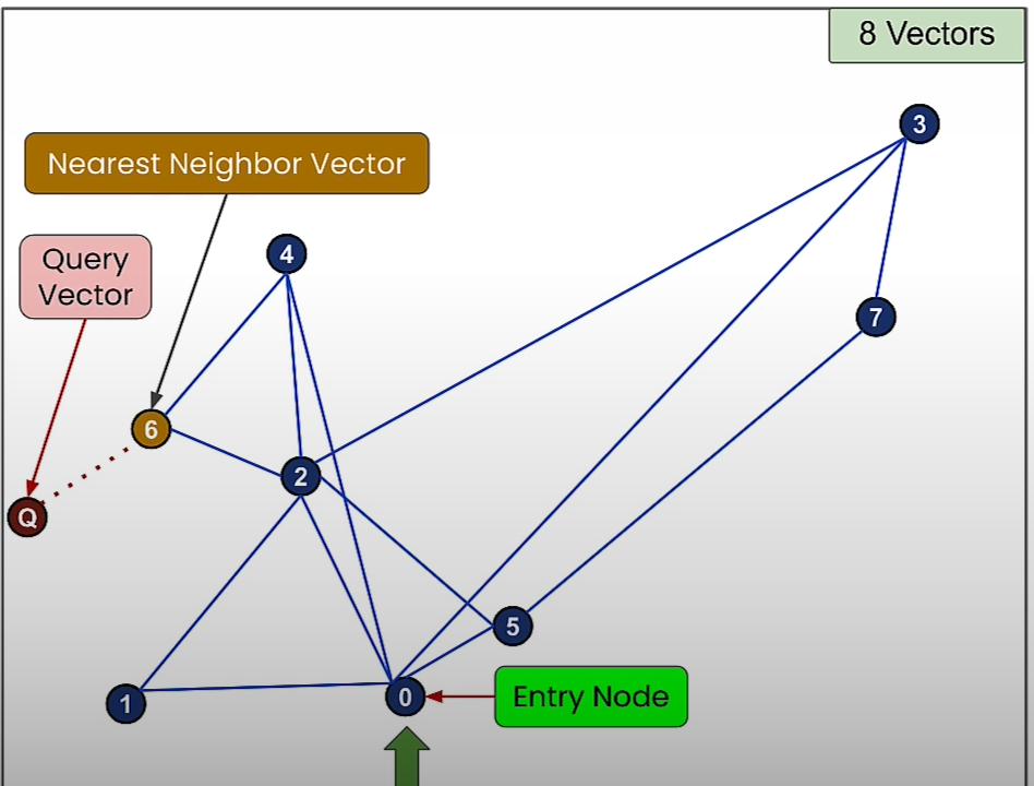
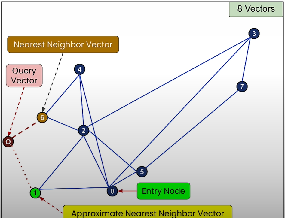
## Query
query_vec = [0.5, 0.5]

nodes = []
nodes.append(("Q",{"pos": query_vec}))

G_query = nx.Graph()
G_query.add_nodes_from(nodes)

print("nodes = ", nodes, flush=True)

pos_query=nx.get_node_attributes(G_query,'pos')

Brute force part:

(G_lin, G_best) = nearest_neigbor(vec_pos,query_vec)

pos_lin=nx.get_node_attributes(G_lin,'pos')
pos_best=nx.get_node_attributes(G_best,'pos')

fig, axs = plt.subplots()

nx.draw(G_lin, pos_lin, with_labels=True, node_size=150, node_color=[[0.8,0.8,1]], width=0.0, font_size=7, ax = axs)
nx.draw(G_query, pos_query, with_labels=True, node_size=200, node_color=[[0.5,0,0]], font_color='white', width=0.5, font_size=7, font_weight='bold', ax = axs)
nx.draw(G_best, pos_best, with_labels=True, node_size=200, node_color=[[0.85,0.7,0.2]], width=0.5, font_size=7, font_weight='bold', ax = axs)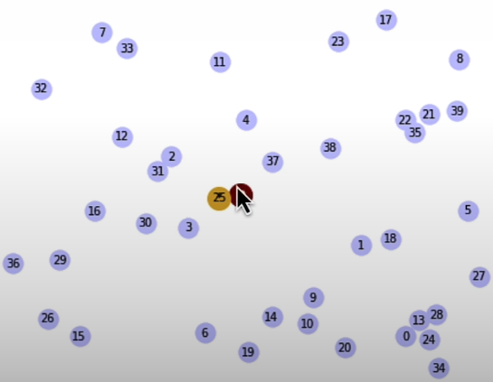

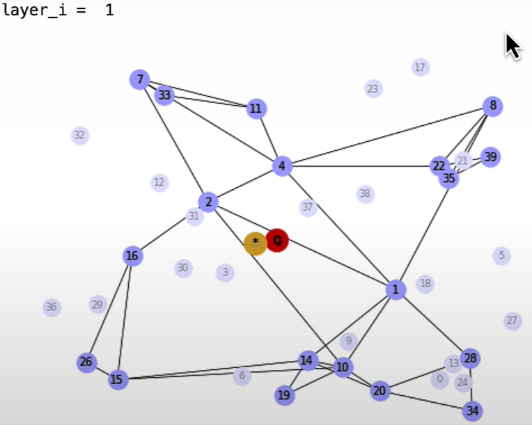
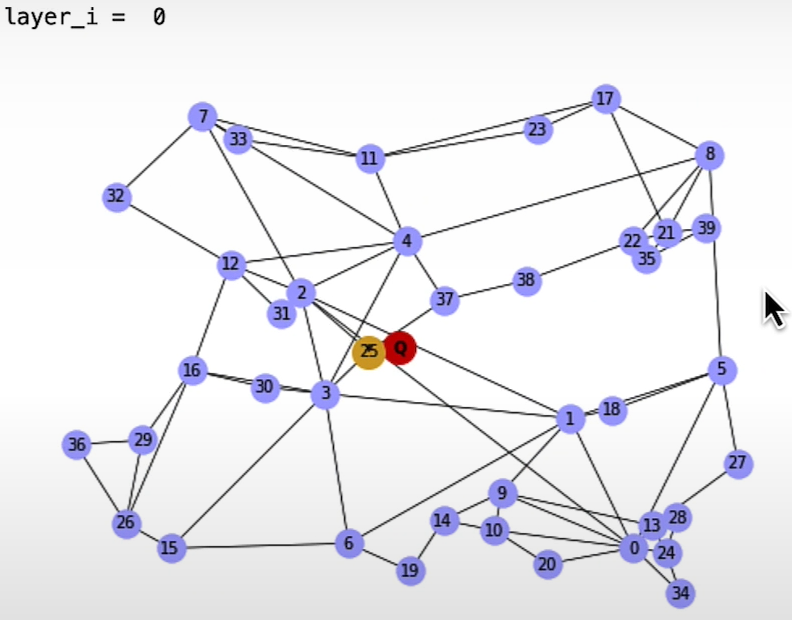
HNSW (Human Navigable Small World)

HNSW also seeks to address this issue and is based on the small world phenomenon of human social networks in which everyone is inextricably linked. The premise is that we are all related by an average of six degrees. So you know a person who knows everyone.

6 Degrees of Seperation

HNSW implementation

HNSW construction:

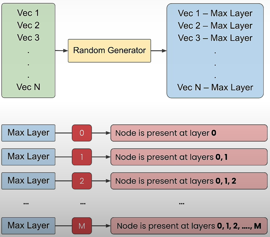
GraphArray = construct_HNSW(vec_pos,m_nearest_neighbor)

for layer_i in range(len(GraphArray)-1,-1,-1):
    fig, axs = plt.subplots()

    print("layer_i = ", layer_i)
        
    if layer_i>0:
        pos_layer_0 = nx.get_node_attributes(GraphArray[0],'pos')
        nx.draw(GraphArray[0], pos_layer_0, with_labels=True, node_size=120, node_color=[[0.9,0.9,1]], width=0.0, font_size=6, font_color=(0.65,0.65,0.65), ax = axs)

    pos_layer_i = nx.get_node_attributes(GraphArray[layer_i],'pos')
    nx.draw(GraphArray[layer_i], pos_layer_i, with_labels=True, node_size=150, node_color=[[0.7,0.7,1]], width=0.5, font_size=7, ax = axs)
    nx.draw(G_query, pos_query, with_labels=True, node_size=200, node_color=[[0.8,0,0]], width=0.5, font_size=7, font_weight='bold', ax = axs)
    nx.draw(G_best, pos_best, with_labels=True, node_size=200, node_color=[[0.85,0.7,0.2]], width=0.5, font_size=7, font_weight='bold', ax = axs)
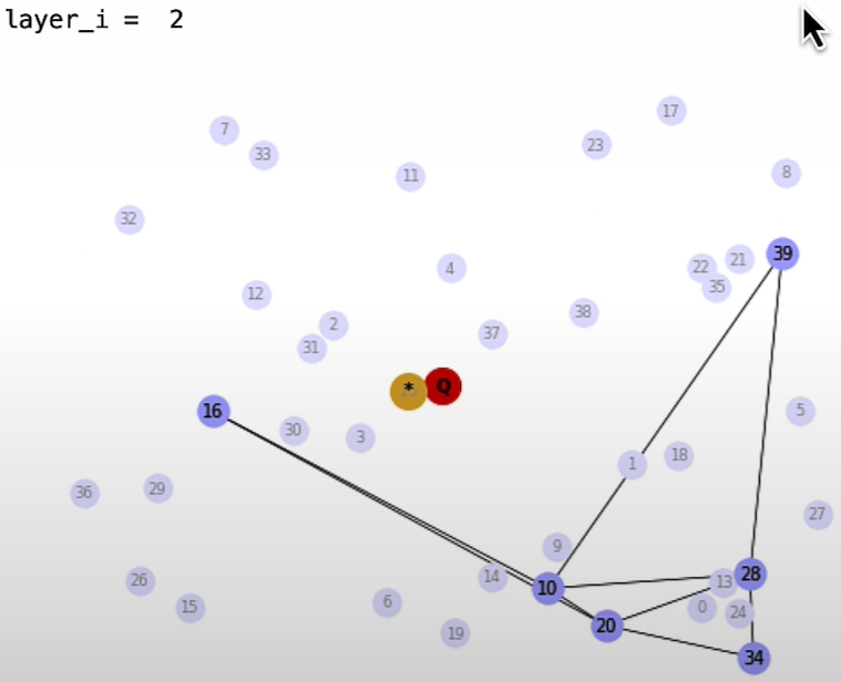
    plt.show()

HNSW Search

HNSW Search Layer 2

HNSW Search Layer 1

HNSW Search Layer 0

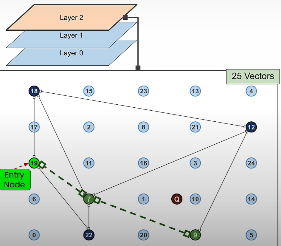
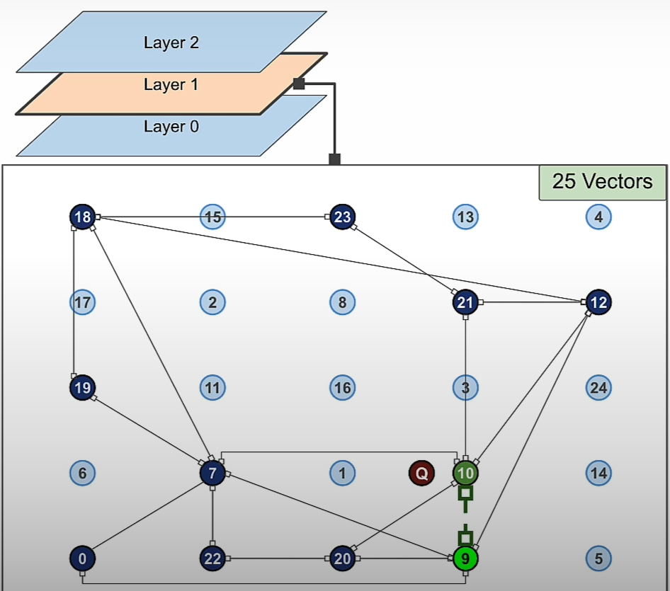
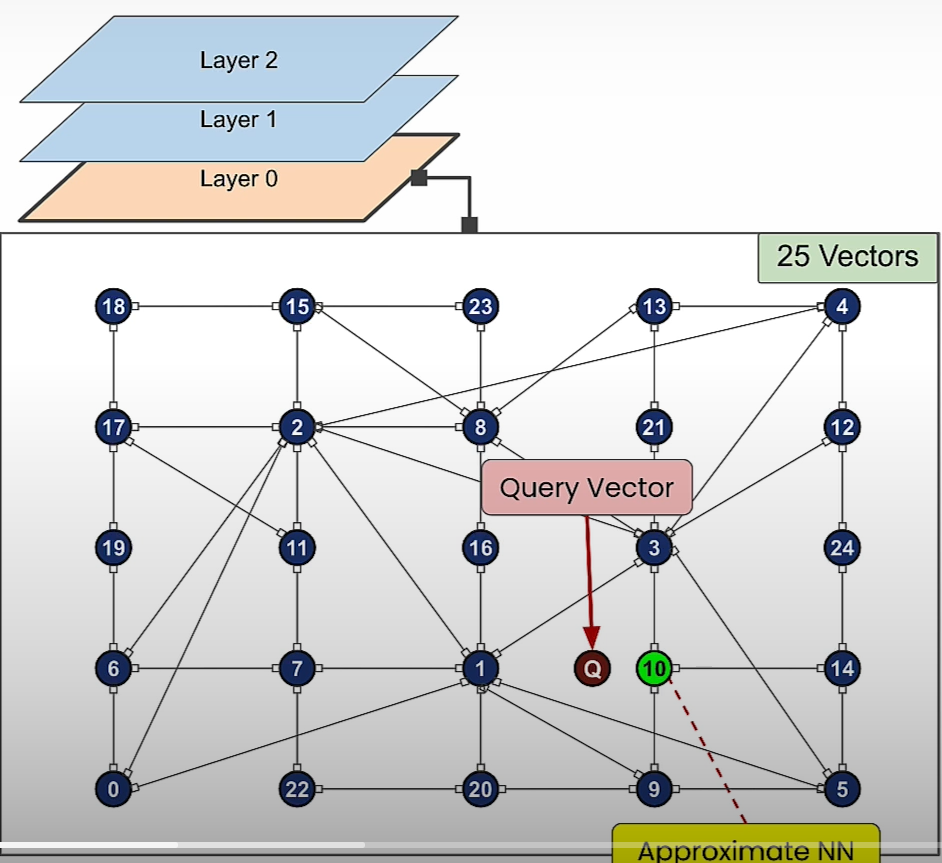
(SearchPathGraphArray, EntryGraphArray) = search_HNSW(GraphArray,G_query)

for layer_i in range(len(GraphArray)-1,-1,-1):
    fig, axs = plt.subplots()

    print("layer_i = ", layer_i)
    G_path_layer = SearchPathGraphArray[layer_i]
    pos_path = nx.get_node_attributes(G_path_layer,'pos')
    G_entry = EntryGraphArray[layer_i]
    pos_entry = nx.get_node_attributes(G_entry,'pos')

    if layer_i>0:
            pos_layer_0 = nx.get_node_attributes(GraphArray[0],'pos')
            nx.draw(GraphArray[0], pos_layer_0, with_labels=True, node_size=120, node_color=[[0.9,0.9,1]], width=0.0, font_size=6, font_color=(0.65,0.65,0.65), ax = axs)

    pos_layer_i = nx.get_node_attributes(GraphArray[layer_i],'pos')
    nx.draw(GraphArray[layer_i], pos_layer_i, with_labels=True, node_size=100, node_color=[[0.7,0.7,1]], width=0.5, font_size=6, ax = axs)
    nx.draw(G_path_layer, pos_path, with_labels=True, node_size=110, node_color=[[0.8,1,0.8]], width=0.5, font_size=6, ax = axs)
    nx.draw(G_query, pos_query, with_labels=True, node_size=80, node_color=[[0.8,0,0]], width=0.5, font_size=7, ax = axs)
    nx.draw(G_best, pos_best, with_labels=True, node_size=70, node_color=[[0.85,0.7,0.2]], width=0.5, font_size=7, ax = axs)
    nx.draw(G_entry, pos_entry, with_labels=True, node_size=80, node_color=[[0.1,0.9,0.1]], width=0.5, font_size=7, ax = axs)
    plt.show()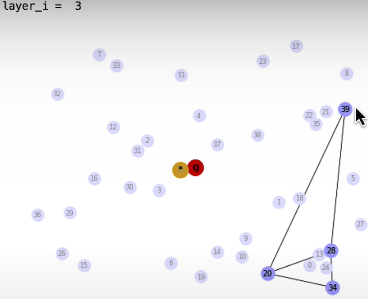

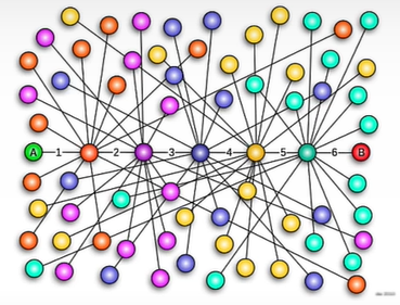
HNSW Search Layer 3

HNSW Search Layer 2

HNSW Search Layer 1

HNSW Search Layer 0

Pure Vector Search — with Weaviate vector database

import weaviate, json
from weaviate import EmbeddedOptions

client = weaviate.Client(
    embedded_options=EmbeddedOptions(),
)

client.is_ready()

# resetting the schema. CAUTION: This will delete your collection 
# if client.schema.exists("MyCollection"):
#     client.schema.delete_class("MyCollection")

schema = {
    "class": "MyCollection",
    "vectorizer": "none",
    "vectorIndexConfig": {
        "distance": "cosine" # let's use cosine distance
    },
}

client.schema.create_class(schema)

print("Successfully created the schema.")

Importing data:

data = [
   {
      "title": "First Object",
      "foo": 99, 
      "vector": [0.1, 0.1, 0.1, 0.1, 0.1, 0.1]
   },
   {
      "title": "Second Object",
      "foo": 77, 
      "vector": [0.2, 0.3, 0.4, 0.5, 0.6, 0.7]
   },
   {
      "title": "Third Object",
      "foo": 55, 
      "vector": [0.3, 0.1, -0.1, -0.3, -0.5, -0.7]
   },
   {
      "title": "Fourth Object",
      "foo": 33, 
      "vector": [0.4, 0.41, 0.42, 0.43, 0.44, 0.45]
   },
   {
      "title": "Fifth Object",
      "foo": 11,
      "vector": [0.5, 0.5, 0, 0, 0, 0]
   },
]

Batch importing data and checking inserts:

client.batch.configure(batch_size=10)  # Configure batch

# Batch import all objects
# yes batch is an overkill for 5 objects, but it is recommended for large volumes of data
with client.batch as batch:
  for item in data:

      properties = {
         "title": item["title"],
         "foo": item["foo"],
      }

      # the call that performs data insert
      client.batch.add_data_object(
         class_name="MyCollection",
         data_object=properties,
         vector=item["vector"] # your vector embeddings go here
      )

# Check number of objects
response = (
    client.query
    .aggregate("MyCollection")
    .with_meta_count()
    .do()
)

print(response)

Query Weaviate — Vector Search (vector embeddings):

response = (
    client.query
    .get("MyCollection", ["title"])
    .with_near_vector({
        "vector": [-0.012, 0.021, -0.23, -0.42, 0.5, 0.5]
    })
    .with_limit(2) # limit the output to only 2
    .do()
)

result = response["data"]["Get"]["MyCollection"]
print(json.dumps(result, indent=2))

response = (
    client.query
    .get("MyCollection", ["title"])
    .with_near_vector({
        "vector": [-0.012, 0.021, -0.23, -0.42, 0.5, 0.5]
    })
    .with_limit(2) # limit the output to only 2
    .with_additional(["distance", "vector, id"])
    .do()
)

result = response["data"]["Get"]["MyCollection"]
print(json.dumps(result, indent=2))

Vector search with filters:

response = (
    client.query
    .get("MyCollection", ["title", "foo"])
    .with_near_vector({
        "vector": [-0.012, 0.021, -0.23, -0.42, 0.5, 0.5]
    })
    .with_additional(["distance, id"]) # output the distance of the query vector to the objects in the database
    .with_where({
        "path": ["foo"],
        "operator": "GreaterThan",
        "valueNumber": 44
    })
    .with_limit(2) # limit the output to only 2
    .do()
)

result = response["data"]["Get"]["MyCollection"]
print(json.dumps(result, indent=2))

nearObject example:

response = (
    client.query
    .get("MyCollection", ["title"])
    .with_near_object({ # the id of the the search object
        "id": result[0]['_additional']['id']
    })
    .with_limit(3)
    .with_additional(["distance"])
    .do()
)

result = response["data"]["Get"]["MyCollection"]
print(json.dumps(result, indent=2))

HNSW Runtime

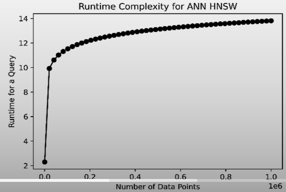
The likelihood of finding a vector at higher altitudes decreases dramatically.

The number of comparisons required to do vector search increases only logarithmically with the quantity of datapoints.

HNSW algorithm has 0(log(N)) runtime complexity.

How to use Weaviate Vector database?

Download sample data

import requests
import json

# Download the data
resp = requests.get('https://raw.githubusercontent.com/weaviate-tutorials/quickstart/main/data/jeopardy_tiny.json')
data = json.loads(resp.text)  # Load data

# Parse the JSON and preview it
print(type(data), len(data))

def json_print(data):
    print(json.dumps(data, indent=2))

json_print(data[0])

Create an embedded instance of Weaviate vector database

import weaviate, os
from weaviate import EmbeddedOptions
import openai

from dotenv import load_dotenv, find_dotenv
_ = load_dotenv(find_dotenv()) # read local .env file
openai.api_key = os.environ['OPENAI_API_KEY']

client = weaviate.Client(
    embedded_options=EmbeddedOptions(),
    additional_headers={
        "X-OpenAI-BaseURL": os.environ['OPENAI_API_BASE'],
        "X-OpenAI-Api-Key": openai.api_key  # Replace this with your actual key
    }
)
print(f"Client created? {client.is_ready()}")
json_print(client.get_meta())

Create Question collection

# resetting the schema. CAUTION: This will delete your collection 
if client.schema.exists("Question"):
    client.schema.delete_class("Question")
class_obj = {
    "class": "Question",
    "vectorizer": "text2vec-openai",  # Use OpenAI as the vectorizer
    "moduleConfig": {
        "text2vec-openai": {
            "model": "ada",
            "modelVersion": "002",
            "type": "text",
            "baseURL": os.environ["OPENAI_API_BASE"]
        }
    }
}

client.schema.create_class(class_obj)

Load sample data and generate vector embeddings

# reminder for the data structure
json_print(data[0])

with client.batch.configure(batch_size=5) as batch:
    for i, d in enumerate(data):  # Batch import data
        
        print(f"importing question: {i+1}")
        
        properties = {
            "answer": d["Answer"],
            "question": d["Question"],
            "category": d["Category"],
        }
        
        batch.add_data_object(
            data_object=properties,
            class_name="Question"
        )

count = client.query.aggregate("Question").with_meta_count().do()
json_print(count)

Let’s Extract the vector that represents each question!

# write a query to extract the vector for a question
result = (client.query
          .get("Question", ["category", "question", "answer"])
          .with_additional("vector")
          .with_limit(1)
          .do())

json_print(result)

Query time

What is the distance between the query: biology and the returned objects?

response = (
    client.query
    .get("Question",["question","answer","category"])
    .with_near_text({"concepts": "biology"})
    .with_additional('distance')
    .with_limit(2)
    .do()
)

json_print(response)

response = (
    client.query
    .get("Question", ["question", "answer"])
    .with_near_text({"concepts": ["animals"]})
    .with_limit(10)
    .with_additional(["distance"])
    .do()
)

json_print(response)

We can let the vector database know to remove results after a threshold distance!

response = (
    client.query
    .get("Question", ["question", "answer"])
    .with_near_text({"concepts": ["animals"], "distance": 0.24})
    .with_limit(10)
    .with_additional(["distance"])
    .do()
)

json_print(response)

CRUD with Weaviate

Create

#Create an object
object_uuid = client.data_object.create(
    data_object={
        'question':"Leonardo da Vinci was born in this country.",
        'answer': "Italy",
        'category': "Culture"
    },
    class_name="Question"
 )

print(object_uuid)

Read

data_object = client.data_object.get_by_id(object_uuid, class_name="Question")
json_print(data_object)

data_object = client.data_object.get_by_id(
    object_uuid,
    class_name='Question',
    with_vector=True
)

json_print(data_object)

Update

client.data_object.update(
    uuid=object_uuid,
    class_name="Question",
    data_object={
        'answer':"Florence, Italy"
    })


data_object = client.data_object.get_by_id(
    object_uuid,
    class_name='Question',
)
json_print(data_object)

Delete

json_print(client.query.aggregate("Question").with_meta_count().do())
client.data_object.delete(uuid=object_uuid, class_name="Question")
json_print(client.query.aggregate("Question").with_meta_count().do())

Sparse, dense and hybrid search

Query Types

Dense Search (Semantic Search)

Searches are performed using vector embedding representations of data.

Example query:

response = (
    client.query
    .get("Question", ["question", "answer"])
    .with_near_text({"concepts":["animal"]})
    .with_limit(3)
    .do()
)

json_print(response)

Dense search shortcomings:

• Out of domain data will provide poor accuracy. 
• Searching for seemingly random data like serial numbers will yield poor accuracy. In this case doing keyword / sparse search will return better results.

The simplest method for keyword matching is to use a bag of words that counts how many times a word appears in the query and the data vector, and then return the objects with the highest matching word frequency.

This is known as sparse search since the text is incorporated in vectors based on how many times each unique word in your vocabulary appears in the query and stored sentences.

Mostly zeroes sparse embeddings

Because the likelihood of any given sentence containing every word in your vocabulary is relatively low, the embeddings are primarily zeros, which is known as a sparse embedding.

BM25 (Best Matching 25)

In practice, while conducting keyword searches, we employ a version of simple word frequencies known as best matching 25. BM25 counts the number of words in the sentence that you are passing in, and those that appear more frequently are weighted as less essential when the match happens, whereas terms that appear infrequently get a much higher score.

Sparse Search — BM25 Example:

response = (
    client.query
    .get("Question",["question","answer"])
    .with_bm25(query="animal")
    .with_limit(3)
    .do()
)

json_print(response)

Hybrid Search

Hybrid search is the process of running both vector/dense and keyword/sparse searches and then integrating the results.

The results can be combined using a scoring system that rates how well each object fits the query in both dense and sparse searches.

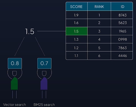
Hybrid search example:

response = (
    client.query
    .get("Question",["question","answer"])
    .with_hybrid(query="animal", alpha=0.5) # Try with alpha= 0.5 and 1 too
    .with_limit(3)
    .do()
)
json_print(response)

Vector Database Utilizing Applications

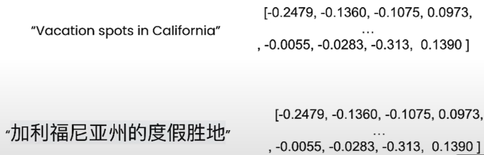
Multilingual or meaning search

Because embedding generates vectors that communicate meaning, vectors representing the same sentence in different languages provide similar outcomes.

Retrieval Augmented Generation (RAG)

Vector databases can be used as an external knowledge base. Allow an LLM to use a vector database as an external knowledge base for factual and updated information.

With RAG, LLMs can cite resources, decrease hallucinations, and complete knowledge-intensive jobs.

To do RAG in Weaviate:

# instruction for the generative module
generatePrompt = "Describe the following as a Facebook Ad: {summary}"

result = (
  client.query
  .get("Article", ["title", "summary"])
  .with_generate(single_prompt=generatePrompt)
  .with_near_text({"concepts": ["Italian food"]})
  .with_limit(5)
).do()

Check stored vector count in database:

print(json.dumps(client.query.aggregate("Wikipedia").with_meta_count().do(), indent=2))

Perform search over them to find concepts you are interested:

response = (client.query
            .get("Wikipedia",['text','title','url','views','lang'])
            .with_near_text({"concepts": "Vacation spots in california"})
            .with_limit(5)
            .do()
           )

json_print(response)

query:

response = (client.query
            .get("Wikipedia",['text','title','url','views','lang'])
            .with_near_text({"concepts": "Vacation spots in california"})
            .with_where({
                "path" : ['lang'],
                "operator" : "Equal",
                "valueString":'en'
            })
            .with_limit(3)
            .do()
           )

json_print(response)


response = (client.query
            .get("Wikipedia",['text','title','url','views','lang'])
            .with_near_text({"concepts": "Miejsca na wakacje w Kalifornii"})
            .with_where({
                "path" : ['lang'],
                "operator" : "Equal",
                "valueString":'en'
            })
            .with_limit(3)
            .do()
           )

json_print(response)

response = (client.query
            .get("Wikipedia",['text','title','url','views','lang'])
            .with_near_text({"concepts": "أماكن العطلات في كاليفورنيا"})
            .with_where({
                "path" : ['lang'],
                "operator" : "Equal",
                "valueString":'en'
            })
            .with_limit(3)
            .do()
           )

json_print(response)

Single prompt:

prompt = "Write me a facebook ad about {title} using information inside {text}"
result = (
  client.query
  .get("Wikipedia", ["title","text"])
  .with_generate(single_prompt=prompt)
  .with_near_text({
    "concepts": ["Vacation spots in california"]
  })
  .with_limit(3)
).do()

json_print(result)

Group Task:

generate_prompt = "Summarize what these posts are about in two paragraphs."

result = (
  client.query
  .get("Wikipedia", ["title","text"])
  .with_generate(grouped_task=generate_prompt) # Pass in all objects at once
  .with_near_text({
    "concepts": ["Vacation spots in california"]
  })
  .with_limit(3)
).do()

json_print(result)

Resource

[1] Deeplearning.ai, (2024), Vector Databases: from Embeddings to Applications:

[https://learn.deeplearning.ai/courses/vector-databases-embeddings-applications/]