What are the quirks of the Python? — Part 3

https://cbarkinozer.medium.com/pythonun-benzersiz-%C3%B6zellikleri-nelerdir-b%C3%B6l%C3%BCm-3-73a23e3bc355

 Part 3 of the quirks of the Python series.

An exception is an error that occurs during the execution of a program. When this problem happens, Python raises an exception that may be addressed, preventing the application from crashing. Exception handling is the process of responding to these mistakes when they occur during program execution. problem handling is often addressed by preserving the execution state at the time the problem occurred and stopping the program’s normal flow to execute a specific function or piece of code known as the exception handler.

Exception handling is accomplished by utilizing built-in programming language exception information objects and/or raising (generating) custom exceptions. Both implementations are quite helpful, and they may be used to do any necessary error checking in your software. In general, built-in exception information is used to detect generic program execution issues, whereas raise exceptions are used to assist with data entry and program conditional validation.

In computer programming, three sorts of mistakes can occur: syntax errors, runtime errors, and logic errors. Syntax errors arise when a program fails to conform to a specified statement of a programming language, preventing the compiler or interpreter from running the source code. Runtime errors occur when a program starts up or during its operation. Logic errors arise when software does not adhere to the established particular requirements that must be met.

When the problem happens, Python raises an exception that can be managed to avoid a crash. Exceptions are used in a variety of ways to handle mistakes and exceptional situations in a program. Now we’ll learn how to retrieve exception information in Python. The built-in “sys.exc_info()” method provides a tuple of three values (type, value, and traceback) that provide information about the exception currently being handled. These parameters indicate the following:

• The type determines the type of exception being handled.
• The value identifies the exception instance type.
• Traceback wraps the call stack at the original exception location.

exception_type, exception_value, exception_traceback = sys.exc_info()

The traceback object stores information about the statement calls performed in your code on a certain line. This object returns a tuple containing the four exception parameters: file name, line number, procedure name, and line code.

exception_type, exception_value, exception_traceback = sys.exc_info()
file_name, line_number, procedure_name, line_code = exception_traceback.extract_tb
(exception_traceback)[-1]

Creating Customized Exceptions

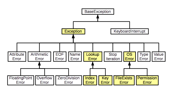
The “BaseException” class is the foundation for all exception classes in Python. The exception is never raised on its own; instead, it should be inherited by other, smaller exception types that can be raised. The “Exception” class is the most typically inherited exception type when building a custom exception class. In general, all exception classes that are deemed errors are subclasses of the Exception type.

“LookupError” is an essential child subclass of the Exception class. This is the basic class for the “IndexError” and “KeyError” classes, which describe the index and key error information, respectively. Custom exception classes should be derived from the built-in classes Exception and IndexError. An exception is a built-in class from which all non-system-exiting exceptions are derived. All user-defined exceptions should be inherited from this class. IndexError is a built-in class. This class raises exceptions when a sequence subscript is out of range.

Handling and Raising Exceptions

Exceptions are handled in Python, like in many other programming languages, by utilizing try-except-finally blocks.

try:
    # Code that may raise an exception
    num1 = int(input("Enter a number: "))
    num2 = int(input("Enter another number: "))
    result = num1 / num2
    print("Result:", result)

except ValueError:
    # Handle the case where input cannot be converted to an integer
    print("Please enter valid integers.")

except ZeroDivisionError:
    # Handle division by zero
    print("Cannot divide by zero.")

finally:
    # This block is always executed, regardless of whether an exception occurred or not
    print("Finally block executed.")

# Continue with the rest of the program
print("Program continues...")

When syntactically valid code encounters a mistake, Python generates an exception error. If an exception occurs, the except block is executed. The “finally” block always appears, regardless of whether an exception occurs.

In real-world business application development, it is useful to write a generic exception-handling method that can be utilized in all custom-developed functions.

def get_exception_details():
    try:
        # Attempt to retrieve information about the current error
        error_type, error_value, error_traceback = sys.exc_info()
        file_name, line_number, function_name, line_code = traceback.extract_tb(error_traceback)[-1]
        # Construct a string containing details about the error
        error_details = ''.join(['[Timestamp]: ', str(time.strftime('%d-%m-%Y %I:%M:%S %p')), 
                                 ' [File]: ', str(file_name), 
                                 ' [Function]: ', str(function_name), 
                                 ' [Error Message]: ', str(error_value), 
                                 ' [Error Type]: ', str(error_type), 
                                 ' [Line Number]: ', str(line_number), 
                                 ' [Line]: ', str(line_code)])
    except:
        # If an error occurs during the retrieval of error information, ignore and continue
        pass
    return error_details

In managing exception block logic, the else clause allows a specific block of code to be executed if no exception occurs.

try:
    # Try to open a file
    file = open("example.txt", "r")
except FileNotFoundError:
    # Handle the case where the file is not found
    print("File not found.")
else:
    # If no exception occurred, read and print the file contents
    print("File opened successfully.")
    print("File contents:")
    print(file.read())
    # Close the file
    file.close()

Raising an Exception

A raise statement has two effects: it either diverts execution to a matching except suite or it terminates the program since no matching except suite could handle the exception. The raise statement accomplishes two things. It generates an exception object and instantly exits the intended program execution sequence to search the enclosing try statements for a matching except clause. The raise statement allows us to cause a specific exception to arise. This enables software engineers to build customized exception messages for specific program situations or implementation needs. In general, this statement can be used within or outside the unless block. This statement has been used in numerous user cases to regulate and validate data.

User-Defined Exceptions 

As we all know, exceptions are Python’s built-in class objects. Based on this, we may design our own custom exception objects by inheriting from them.

class CustomException(Exception):
    def __init__(self, parameter, message):
        self.parameter = parameter
        self.message = message
        super().__init__(self.message)

# Example usage:
def validate_age(age):
    if age < 0:
        raise CustomException(age, "Age cannot be negative.")

try:
    user_age = int(input("Enter your age: "))
    validate_age(user_age)
    print("Valid age entered:", user_age)
except CustomException as e:
    print("Custom Exception:", e.message)
    print("Parameter:", e.parameter)

Common Libraries

The Python libraries contain both the default core libraries from the distribution package and the data ecosystem libraries, which are primarily designed for data analytics and machine learning/artificial intelligence projects. Python is one of the most popular programming languages today, thanks to these 1000+ created libraries. Because all of the libraries are open-source, we’ve included contributions, contributor counts, and other data from Github, which might serve as a proxy statistic for library popularity. According to my recent experience, the most significant and relevant libraries for data scientists and data engineers are NumPy, pandas, matplotlib, SymPy, IPython, SciPy, Seaborn, scikit-learn, and Bokkeh. These libraries are widely used in machine learning and artificial intelligence research.

Today, software engineers and data scientists must prioritize the speeding up of Python projects. The most frequent libraries for speeding up Python code are Cython, PyPy, and Numba. It is vital to note that Numba is now the most popular program for speeding up Python programs. Python’s data visualization libraries include Matplotlib, Seaborn, and Bokeh. Data visualization is a critical stage in every statistical analysis or machine learning endeavour. Accessing database engines with Python is a critical prerequisite for designing and developing database business applications nowadays. The SQLAlchemy SQL toolkit is the most common database library for these scenarios.

Standard Python Library

The Python standard library comprises of reusable built-in module files that may be loaded into your programs. They are included in the main Python distribution package. Python offers more than 200 standard libraries. These libraries are written in the C language. Aside from this standard library, a large international community of people and corporations is constantly producing bespoke Python libraries. The Python Data Ecosystem includes more than 1000 developed libraries.

The following are the most prominent data ecosystem libraries used in Python today:

• NumPy is abbreviated as Numerical Python. It is a core package for scientific computing. This may be the most significant library in the Python programming language right now.
• Pandas is an open-source framework that offers high-performance, user-friendly data structures and analysis tools.
• Matplotlib is a Python 2D plotting package that generates publication-quality figures in a range of hardcopy and interactive formats on several platforms.
• SymPy is a library designed for symbolic mathematics. It intends to become a full-featured computer algebra system (CAS) while keeping the code as basic as possible so that it is understandable and adaptable. SymPy was developed entirely in Python.
• IPython is a comprehensive interactive computing architecture that includes a robust interactive shell, a Jupyter kernel, and support for interactive data visualization and GUI toolkits. It also contains versatile, embeddable interpreters that you may use in your own projects, as well as simple, high-performance parallel computing tools.
• SciPy is a Python-based environment for open-source software in mathematics, science, and engineering. Some of the core packages are NumPy, SciPy library, matplotlib, IPython, SymPy, and pandas.
• Seaborn is a Python data visualization package built on matplotlib. It provides a high-level interface for creating visually appealing and useful statistical graphs.
• Scikit-learn is the primary machine learning framework. It’s a simple and effective tool for data mining and analysis. This framework is based on the NumPy, SciPy, and Matplotlib packages.
• Bokkeh is an interactive visualization library for current web browsers. Its purpose is to deliver attractive, concise development of adaptable visuals while also extending this capacity with high-performance interactivity over very large or streaming information.

Scientific Calculations

Scientific computations are always required for research initiatives and business application development nowadays. Python is a fantastic choice for scientific computations since it has a large international user base, is simple to develop and find, and offers a rich ecosystem of scientific and technical resources. Python is also known for its great performance, which is owing to highly optimized C code, outstanding software, hardware support for parallel processing, and the fact that Python is an open-source software licensed under the Python Software Foundation.

NumPy

Almost all numerical operations in Python are performed using the NumPy package. NumPy could be considered the most important library in the Python Data Ecosystem bundle. It offers high-performance vector, matrix, and higher-dimensional data structures in Python. It is developed in C and FORTRAN, which means that when math operations are performed using vectors and matrices, the performance is excellent.

import numpy as np

# Alice's scores
alice_scores = np.array([85, 90, 75, 88, 92])

# Bob's scores
bob_scores = np.array([78, 85, 80, 82, 90])

# Calculate the correlation coefficient between Alice's and Bob's scores
np_corrcoef = np.corrcoef(alice_scores, bob_scores)
print("Correlation Coefficient between Alice's and Bob's scores:")
print(np_corrcoef)

# Calculate the mean score for Alice
np_mean_alice = np.mean(alice_scores)
print("Mean score for Alice:", np_mean_alice)

# Calculate the mean score for Bob
np_mean_bob = np.mean(bob_scores)
print("Mean score for Bob:", np_mean_bob)

# Calculate the average score for Alice (same as mean in this context)
np_average_alice = np.average(alice_scores)
print("Average score for Alice:", np_average_alice)

# Calculate the standard deviation of scores for Alice
np_std_alice = np.std(alice_scores)
print("Standard Deviation of scores for Alice:", np_std_alice)

# Calculate the median score for Alice
np_median_alice = np.median(alice_scores)
print("Median score for Alice:", np_median_alice)

# Calculate the variance of scores for Alice
np_variance_alice = np.var(alice_scores)
print("Variance of scores for Alice:", np_variance_alice)

# Find the highest score Alice achieved
np_max_alice = np.max(alice_scores)
print("Highest score for Alice:", np_max_alice)

# Find the lowest score Alice achieved
np_min_alice = np.min(alice_scores)
print("Lowest score for Alice:", np_min_alice)

# Calculate the sum of scores for Alice
np_sum_alice = np.sum(alice_scores)
print("Sum of scores for Alice:", np_sum_alice)

On a structural level, an array is simply a collection of pointers. It consists of a memory address, data type, shape, and strides. These aspects of an array have the following characteristics:

• The data pointer represents the memory address of the first byte in the array.
• The data type, also known as the type pointer, describes the type of components that make up the array.
• The shape indicates the array’s shape.
• The strides are the number of bytes that should be skipped in memory before proceeding to the next element. If your strides are (100,1), you need to move one byte to the next column and 100 bytes to the next row.

There are two methods for installing Python libraries:

• To install a “library_name” using PyPI (pip), use “pip install library_name” or “python -m pip install — upgrade library_name”.
• To install a library, use the “conda” command from the Anaconda Distribution package and type “conda install library_name” on the command prompt.

Pandas

The pandas package is the primary data structure and processing tool in Python. It is developed on top of the NumPy library, which means that many NumPy structures are used or duplicated in the pandas library. This can be applied to data analysis and visualization. Pandas library supports a variety of data kinds, including heterogeneous data types, easy and quick handling of missing data, generic code that is simple to create, labeled data, and relational data. This package is widely used in machine learning applications for data loading, preprocessing (cleaning), and profiling.

Pandas Series

This is a one-dimensional labeled array that can contain any data type, including integers, texts, floating-point numbers, Python objects, and so on. The axis labels are collectively known as the index. A series can be built using the following syntax, with “data” being a Python dictionary, ndarray (n-dimensional array or any scalar value), and so on.

serie = pd.Series(np.random.randn(5))

DataFrames are two-dimensional labeled data structures with rows and columns containing the same or distinct data kinds. It is similar to Microsoft Excel spreadsheets and SQL database table objects. The first column of this component is allocated for index values. If these values are not defined, pandas will create integers that begin with zero. This component is currently the most useful in machine learning applications for data manipulation. The code below explains how to construct a pandas DataFrame object.

# Example data
data = {'Name': ['Alice', 'Bob', 'Charlie', 'David'],
        'Age': [25, 30, 35, 40],
        'City': ['New York', 'Los Angeles', 'Chicago', 'Houston']}

# Creating a Pandas DataFrame from the dictionary
df_data = pd.DataFrame(data)

The DataFrame can accept a wide range of input data types, including 1D or 2D NumPy arrays, lists, dictionaries, tuples, structured or record ndarrays, series, and other DataFrame objects.

It is critical to note that axis labelling information in pandas objects serves a variety of functions, including data identification using defined indicators for profiling, visualization, and analysis, automatic and explicit data alignment, and fast data retrieval by obtaining and setting dataset subsets. One of the most common tasks in scientific computations for data analytics is reading data from a comma-separated value (CSV) file. This file delimits plain text data with commas to separate values.

df = pd.read_csv(filepath_or_buffer="input_with_nan.csv")

It’s worth noting that pandas treats empty values with a float-defined value as nota-number (NaN). This value is neither empty, null, or equal to zero. The Pandas library contains a number of methods for properly handling these values during data manipulation. These values will not be used in any computer calculations.

Pandas example:

import pandas as pd
import numpy as np
from datetime import datetime

# Create a sample DataFrame
data = {'Column1': [1, 2, np.nan, 4],
        'Column2': [np.nan, 6, np.nan, 8],
        'Column3': [10, np.nan, 30, 40],
        'Column4': ['', 'club', np.nan, ''],
        'Column5': [True, np.nan, False, np.nan],
        'Column6': ['', '', np.nan, ''],
        'Column7': [100, np.nan, 300, np.nan],
        'Column8': ['£100', '£200', '£300', '£400']}

df = pd.DataFrame(data)

# Drop duplicated rows and keep the first
df = df.drop_duplicates()

# Replace empty values with the mean value in columns 1 and 2
df['Column1'].fillna(df['Column1'].mean(), inplace=True)
df['Column2'].fillna(df['Column2'].mean(), inplace=True)

# Replace empty values with the median value in column 3
df['Column3'].fillna(df['Column3'].median(), inplace=True)

# Replace empty values with the “club” string in column 4
df['Column4'].fillna('club', inplace=True)

# Replace empty values with the true boolean in column 5
df['Column5'].fillna(True, inplace=True)

# Replace empty values with the current date in column 6
df['Column6'].fillna(datetime.today().strftime('%Y-%m-%d'), inplace=True)

# Replace empty values with the £0.0 in column 7
df['Column7'].fillna(0.0, inplace=True)

# Remove the first character (English pound symbol) in column 8
df['Column8'] = df['Column8'].str[1:]

# Substitute the abbreviation in column 8
df['Column8'] = df['Column8'].replace({'100': 'Hundred', '200': 'Two Hundred', '300': 'Three Hundred', '400': 'Four Hundred'})

# Define x column labels
x_column_labels = ['Column1', 'Column2', 'Column3', 'Column4', 'Column5', 'Column6', 'Column7', 'Column8']

# Define y column target
y_column_target = 'Column8'

# Save the final file as “output_data.csv”. File location path must be defined.
output_file_path = "output_data.csv"
df.to_csv(output_file_path, index=False)

# Display the final DataFrame
print("Final DataFrame after operations:")
print(df)

SciPy

SciPy is a popular Python scientific algorithm library. It extends the low-level NumPy library for one-dimensional and multidimensional arrays. This library includes a huge number of higher-level scientific algorithms in Python.

Some of the main sublibraries are:

• special functions
• integration
• optimization
• interpolation
• Fourier transforms
• signal processing
• linear algebra
• sparse eigenvalue problems
• statistics
• multi-dimensional image processing
• file IO

Scipy example:

import numpy as np
from scipy import optimize, interpolate, integrate, stats, linalg, special

# Optimization: find the minimum of a function
def func(x):
    return x**2 + 10*np.sin(x)

min_result = optimize.minimize(func, x0=0)
print("Optimization result:")
print(min_result)

# Interpolation: interpolate data points using linear and cubic functions
x = np.array([0, 1, 2, 3, 4])
y = np.array([0, 1, 4, 9, 16])

# Linear interpolation
f_linear = interpolate.interp1d(x, y)
x_linear = np.linspace(0, 4, 10)
y_linear = f_linear(x_linear)

# Cubic interpolation
f_cubic = interpolate.interp1d(x, y, kind='cubic')
y_cubic = f_cubic(x_linear)

print("\nInterpolated data (linear and cubic):")
print("Linear:", list(zip(x_linear, y_linear)))
print("Cubic:", list(zip(x_linear, y_cubic)))

# Integration: compute definite integral of a function
result_integral = integrate.quad(lambda x: np.sin(x), 0, np.pi)
print("\nDefinite integral result:")
print(result_integral)

# Statistics: compute mean, median, mode, and standard deviation
data = np.random.normal(loc=0, scale=1, size=100)
mean = np.mean(data)
median = np.median(data)
mode = stats.mode(data)
std_dev = np.std(data)
print("\nStatistics results:")
print("Mean:", mean)
print("Median:", median)
print("Mode:", mode)
print("Standard Deviation:", std_dev)

# Linear algebra: solve a system of linear equations
A = np.array([[2, 1], [1, 1]])
b = np.array([1, 1])
x_solution = linalg.solve(A, b)
print("\nSolution to the system of linear equations:")
print(x_solution)

# Bessel functions: evaluate the first and second Bessel functions
x_values = np.linspace(0, 10, 100)
bessel_first = special.jn(1, x_values)
bessel_second = special.jn(2, x_values)
print("\nValues of the first and second Bessel functions:")
print("First Bessel:", bessel_first)
print("Second Bessel:", bessel_second)